13 CFA and SEM with lavaan
13.1 Confirmatory factor analysis (CFA)
lavaan is a free open source package for latent variable modeling in R. The package is developed and maintained by Yves Rosseel (Rosseel, 2012; see also http://lavaan.ugent.be). The name lavaan refers to latent variable analysis.
lavaan can be used to estimate a variety of statistical models: path analysis, structural equation models (SEM) and confirmatory factor analyses (CFA).
13.1.1 Setup: Packages and data
pacman::p_load(tidyverse, ggm, ggplot2, ggthemes, haven, lavaan, lavaanPlot, knitr, psych, semPlot, semTools, wesanderson)lifesat <- read_csv(
url("https://raw.githubusercontent.com/methodenlehre/data/master/lifesat.csv"))## Rows: 275 Columns: 13## ── Column specification ────────────────────────────────────────────────────────
## Delimiter: ","
## chr (1): gender
## dbl (12): ID, age, school1, school2, school3, self1, self2, friends1, friend...##
## ℹ Use `spec()` to retrieve the full column specification for this data.
## ℹ Specify the column types or set `show_col_types = FALSE` to quiet this message.# convert ID and gender to factors
lifesat$ID <- as.factor(lifesat$ID)
lifesat$gender <- as.factor(lifesat$gender)The life satisfaction data consist of 10 items related to different aspects/domains of life satisfaction. The adolescents were asked:
“How satisfied are you with…?”
| Items | |
|---|---|
| school1 | your school grade |
| school2 | your relationship with your teacher |
| school3 | your school life |
| self1 | your looks and appearance |
| self2 | your personality |
| friends1 | your social life |
| friends2 | your relationships with your friends |
| fam1 | your relationship with your parents |
| fam2 | your family life |
| fam3 | your socio-economic status |
The response was on a 7-point scale from 1 = “not satisfied at all” to 7 = “very satisfied”.
The questions on life satisfaction can be divided into four domains: school, self, friends, family
The ML estimation assumes a multivariate normal distribution. Let’s first look at the univariate skewness and kurtosis using describe() from psych:
check_cfa <- lifesat[-(1:3)] %>%
  describe()

check_cfa$skew
## [1] -0.7159340 -0.7609000 -0.6756997 -1.0303710 -1.5071008 -1.2017037
## [7] -0.8989515 -1.6183389 -1.4575230 -1.4230322check_cfa$kurtosis## [1] 0.2828551 0.8154313 0.2107045 1.1177822 3.7815521 3.5733595 0.4539949
## [8] 3.0151001 3.0209721 3.1563637Serious deviations from the normal distribution are present if the skewness of the manifest variables is greater than an absolute value of 2 and the (excess) kurtosis is greater than 4.
We can check multivariate skewness and kurtosis (Mardia’s coefficients):
lifesat[-(1:3)] %>%
mardiaSkew()
## b1d chi df p
## 2.832089e+01 1.298041e+03 2.200000e+02 3.893895e-152lifesat[-(1:3)] %>%
mardiaKurtosis()## b2d z p
## 1.842232e+02 3.437339e+01 6.300872e-259According to these cutoffs our items do not seem to be very problematic univariately, but both multivariate skewness and kurtosis are very high, pointing to multivariate outliers that might inflate standard errors of coefficients (coefficients themselves are mostly unaffected by non-normality).
We will therefore request additional estimation methods as well as bootstrap analysis to account for non-normality.
13.1.2 Defining the CFA model in lavaan
The calculation of a CFA with lavaan is done in two steps:
A model defining the hypothesized factor structure is set up
This model is estimated using
cfa(), which takes as input both the data and the model definition. Model definitions inlavaanall follow the same type of syntax.
In the model definition syntax, certain characters (operators) are predefined and a number of default settings are applied. For example, by default the scaling of the latent variable is achieved by fixing the loading of the first indicator (manifest variable) for a latent variable to the value of 1.
=~ indicates that the latent variable (here named Factor1) to the left of the operator is defined by all variables to the right of it. The manifest (measured) variables from the dataset on the right are separated by a +.
An example of six items explained by two factors (latent variables):
example_model <- "
Factor1 =~ var1 + var2 + var3
Factor2 =~ var4 + var5 + var6
# The order of the manifest variables is relevant only for fixing one loading per factor.
# Here the loadings of `var1` and `var4` are set to the value 1.

# Comments like this are ignored by lavaan.
"
The parameters of the model do not have to be explicitly defined (e.g. l12 for the loading of the second item (var2) on the first factor (Factor1). However, they can be defined explicitly and we will see that this will be necessary in some situations.
Another default is that factor variances and covariances are automatically specified for all latent variables in a CFA. The operator for specifying a variance/covariance is ~~. Variances are defined as covariances of a variable with itself. Thus, in this example we could add the lines Factor1 ~~ Factor1, Factor2 ~~ Factor2 (latent variable variances), and Factor1 ~~ Factor2 (latent variable covariance) without changing the model definition. The same holds for the residual variances of the manifest variables (but not for potential residual covariances!).
13.1.3 Estimating the model
Syntax for estimation:
cfa(model = example_model, data = dataframe)
The direct execution of this syntax results in only a very limited output, containing only the number of estimated parameters, the number of observations, and the chi-square statistics.
Therefore, like with lm() the result of cfa() must first be assigned to an output object (e.g. fit_example_model) and the detailed output (including the parameter estimates) extracted with summary().
Additional arguments of the summary() function : fit.measures = TRUE returns a number of global fit indices (e.g. SRMR, RMSEA, CLI, TLI) as well as information criteria (e.g. AIC and BIC), and with standardized = TRUE we obtain both the unstandardized and the standardized parameter estimates.
13.1.4 Life satisfaction CFA with four factors
For theoretical reasons, we first estimate a model with four factors. We define one factor for each content domain of life satisfaction (school, self, friends, family). In addition, as usual we postulate a simple structure, i.e. all potential cross-loadings are restricted to the value of 0 (i.e., in the model definition manifest variables only appear once - in the equation of their respective factor).
The theoretical model looks like this:
semPaths(fit_mod4f)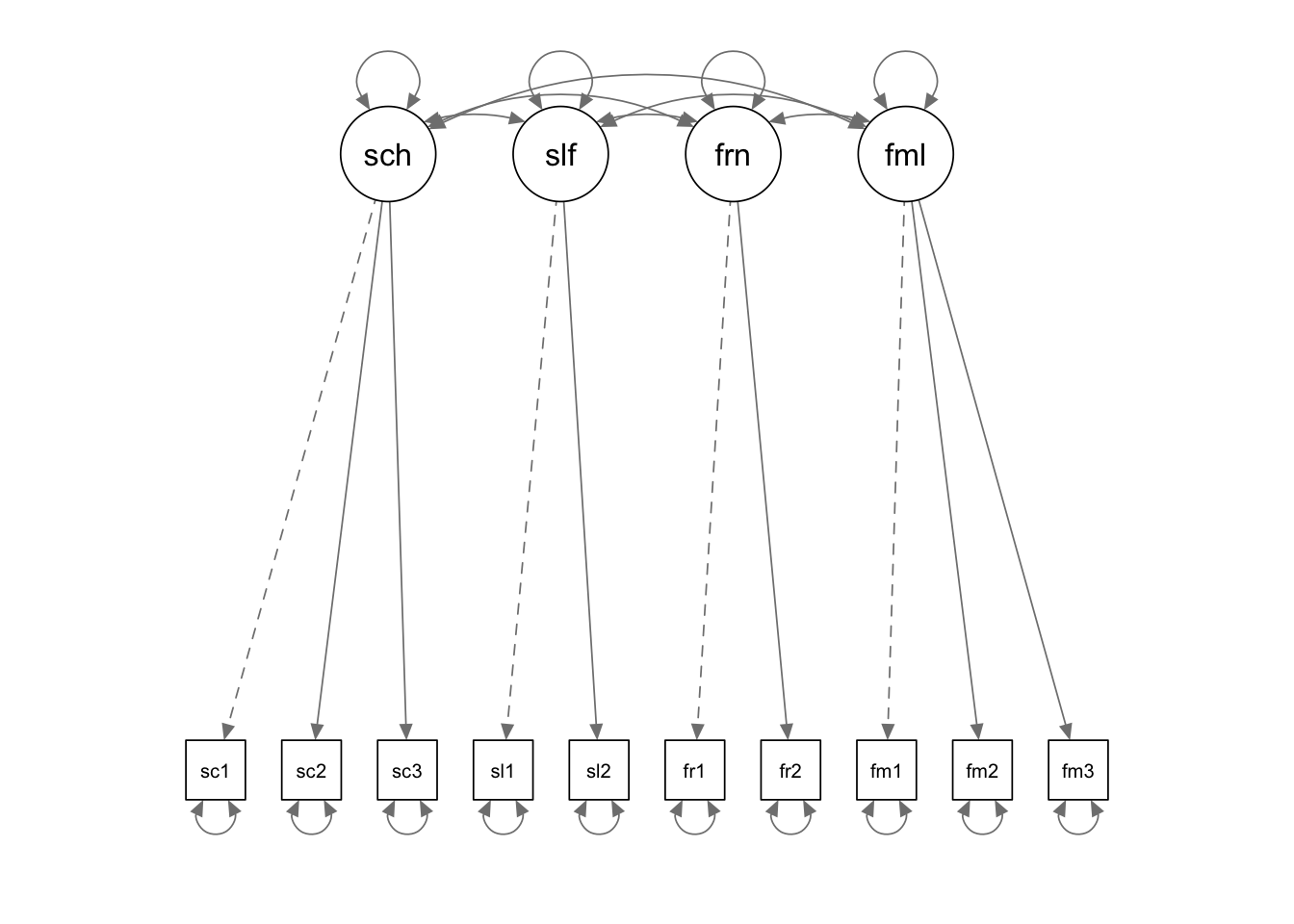
Modell definition
model_4f <- "
school =~ school1 + school2 + school3
self =~ self1 + self2
friends =~ friends1 + friends2
family =~ fam1 + fam2 + fam3
"
Model estimation
Because of the multivariate non-normality of the data we use an alternative maximum-likelihood estimation method - robust ML. As noted above the parameter estimates themselves are usually unbiased also under non-normality but the standard errors are not.
Thus, we estimate the parameters with regular ML but with robust (and therefore greater) standard errors that correct for non-normality (se = "robust").
Furthermore, we use a robust scaled chi-square test statistic (test = "Satorra-Bentler") that corrects for the fact that for non-normal data the usual model test statistic tends to be too large. The Satorra-Bentler test rescales the value of the ML chi-square test according to the degree of multivariate kurtosis of the data.
The combination of se = "robust" and test = "Satorra-Bentler" can be called with estimator = "MLM:
fit_mod4f <- cfa(model_4f,
                 data = lifesat,
                 estimator = "MLM")

semPaths(fit_mod4f, "std")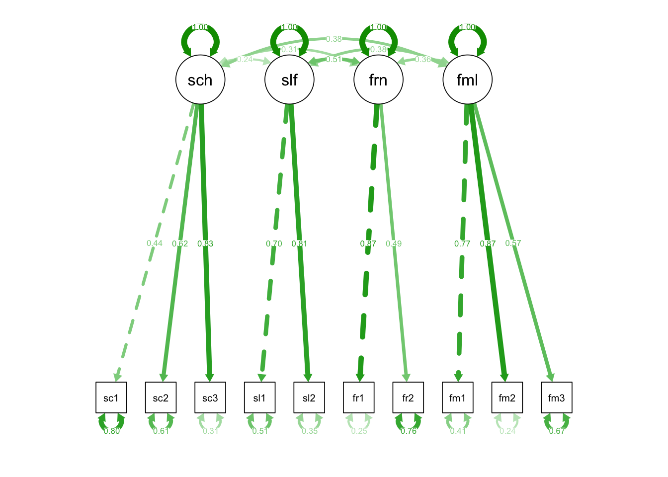
summary(fit_mod4f, fit.measures = TRUE, standardized = TRUE)## lavaan 0.6-9 ended normally after 46 iterations
##
## Estimator ML
## Optimization method NLMINB
## Number of model parameters 26
##
## Number of observations 275
##
## Model Test User Model:
## Standard Robust
## Test Statistic 68.209 47.000
## Degrees of freedom 29 29
## P-value (Chi-square) 0.000 0.019
## Scaling correction factor 1.451
## Satorra-Bentler correction
##
## Model Test Baseline Model:
##
## Test statistic 725.606 420.551
## Degrees of freedom 45 45
## P-value 0.000 0.000
## Scaling correction factor 1.725
##
## User Model versus Baseline Model:
##
## Comparative Fit Index (CFI) 0.942 0.952
## Tucker-Lewis Index (TLI) 0.911 0.926
##
## Robust Comparative Fit Index (CFI) 0.960
## Robust Tucker-Lewis Index (TLI) 0.937
##
## Loglikelihood and Information Criteria:
##
## Loglikelihood user model (H0) -4064.982 -4064.982
## Loglikelihood unrestricted model (H1) -4030.877 -4030.877
##
## Akaike (AIC) 8181.964 8181.964
## Bayesian (BIC) 8276.000 8276.000
## Sample-size adjusted Bayesian (BIC) 8193.559 8193.559
##
## Root Mean Square Error of Approximation:
##
## RMSEA 0.070 0.048
## 90 Percent confidence interval - lower 0.049 0.025
## 90 Percent confidence interval - upper 0.092 0.068
## P-value RMSEA <= 0.05 0.061 0.556
##
## Robust RMSEA 0.057
## 90 Percent confidence interval - lower 0.024
## 90 Percent confidence interval - upper 0.086
##
## Standardized Root Mean Square Residual:
##
## SRMR 0.059 0.059
##
## Parameter Estimates:
##
## Standard errors Robust.sem
## Information Expected
## Information saturated (h1) model Structured
##
## Latent Variables:
## Estimate Std.Err z-value P(>|z|) Std.lv Std.all
## school =~
## school1 1.000 0.635 0.444
## school2 1.300 0.279 4.669 0.000 0.826 0.625
## school3 1.834 0.357 5.144 0.000 1.165 0.830
## self =~
## self1 1.000 0.924 0.700
## self2 0.993 0.164 6.058 0.000 0.917 0.806
## friends =~
## friends1 1.000 0.886 0.869
## friends2 0.453 0.148 3.059 0.002 0.401 0.494
## family =~
## fam1 1.000 1.017 0.769
## fam2 1.051 0.149 7.048 0.000 1.069 0.872
## fam3 0.629 0.117 5.399 0.000 0.640 0.572
##
## Covariances:
## Estimate Std.Err z-value P(>|z|) Std.lv Std.all
## school ~~
## self 0.141 0.065 2.167 0.030 0.240 0.240
## friends 0.177 0.056 3.158 0.002 0.315 0.315
## family 0.246 0.072 3.427 0.001 0.381 0.381
## self ~~
## friends 0.419 0.092 4.563 0.000 0.512 0.512
## family 0.355 0.129 2.754 0.006 0.378 0.378
## friends ~~
## family 0.321 0.111 2.888 0.004 0.356 0.356
##
## Variances:
## Estimate Std.Err z-value P(>|z|) Std.lv Std.all
## .school1 1.639 0.177 9.249 0.000 1.639 0.803
## .school2 1.066 0.207 5.143 0.000 1.066 0.610
## .school3 0.613 0.281 2.180 0.029 0.613 0.311
## .self1 0.886 0.172 5.159 0.000 0.886 0.510
## .self2 0.453 0.175 2.595 0.009 0.453 0.350
## .friends1 0.255 0.218 1.173 0.241 0.255 0.245
## .friends2 0.499 0.060 8.285 0.000 0.499 0.756
## .fam1 0.714 0.152 4.685 0.000 0.714 0.408
## .fam2 0.359 0.119 3.029 0.002 0.359 0.239
## .fam3 0.842 0.121 6.944 0.000 0.842 0.672
## school 0.403 0.120 3.369 0.001 1.000 1.000
## self 0.853 0.212 4.016 0.000 1.000 1.000
## friends 0.784 0.276 2.842 0.004 1.000 1.000
## family 1.035 0.228 4.533 0.000 1.000 1.000Local model fit: Comparing the empirical and implied variance-covariance matrix
The lavInspect() function allows extracting information from a lavaan object. The argument what specifies which information should be extracted. The value sampstat of this argument stands for “sample statistics”, the empirical variance-covariance matrix:
lavInspect(fit_mod4f, what = "sampstat")## $cov
## schol1 schol2 schol3 self1 self2 frnds1 frnds2 fam1 fam2 fam3
## school1 2.042
## school2 0.473 1.748
## school3 0.705 0.990 1.969
## self1 0.305 0.240 0.409 1.739
## self2 0.262 0.040 0.182 0.847 1.294
## friends1 0.261 0.108 0.375 0.369 0.437 1.039
## friends2 0.037 0.063 0.094 0.167 0.221 0.356 0.660
## fam1 0.543 0.231 0.434 0.437 0.385 0.307 0.189 1.749
## fam2 0.540 0.327 0.369 0.378 0.261 0.331 0.150 1.103 1.502
## fam3 0.353 0.314 0.391 0.477 0.369 0.231 0.103 0.575 0.693 1.252The variance-covariance matrix implied by the model is obtained with what = "implied":
lavInspect(fit_mod4f, what = "implied")## $cov
## schol1 schol2 schol3 self1 self2 frnds1 frnds2 fam1 fam2 fam3
## school1 2.042
## school2 0.525 1.748
## school3 0.740 0.962 1.969
## self1 0.141 0.183 0.258 1.739
## self2 0.140 0.182 0.256 0.847 1.294
## friends1 0.177 0.230 0.324 0.419 0.416 1.039
## friends2 0.080 0.104 0.147 0.190 0.189 0.356 0.660
## fam1 0.246 0.320 0.452 0.355 0.352 0.321 0.145 1.749
## fam2 0.259 0.337 0.475 0.373 0.370 0.337 0.153 1.088 1.502
## fam3 0.155 0.202 0.284 0.223 0.222 0.202 0.092 0.651 0.685 1.252The smaller the differences between these two matrices, the better the model fits the data. In other words, the closer are the variances and covariances recalculated from the estimated parameters to the empirical variances and covariances.
The residual matrix results from the subtraction of the variance-covariance matrix implied by the model from the observed (empirical) variance-covariance matrix.
residual_matrix <-
  lavInspect(fit_mod4f, what = "sampstat")$cov -
  lavInspect(fit_mod4f, what = "implied")$cov

residual_matrix
## schol1 schol2 schol3 self1 self2 frnds1 frnds2 fam1 fam2 fam3
## school1 0.000
## school2 -0.052 0.000
## school3 -0.035 0.028 0.000
## self1 0.164 0.057 0.151 0.000
## self2 0.122 -0.141 -0.074 0.000 0.000
## friends1 0.084 -0.122 0.051 -0.050 0.021 0.000
## friends2 -0.043 -0.042 -0.053 -0.022 0.033 0.000 0.000
## fam1 0.296 -0.090 -0.018 0.082 0.033 -0.014 0.044 0.000
## fam2 0.281 -0.009 -0.106 0.005 -0.110 -0.006 -0.003 0.015 0.000
## fam3 0.198 0.113 0.107 0.254 0.147 0.029 0.011 -0.076 0.008 0.000A direct extraction of the residual matrix can be obtained with the argument what = "resid":
lavInspect(fit_mod4f, what = "resid")## $cov
##          schol1 schol2 schol3 self1  self2  frnds1 frnds2 fam1   fam2   fam3
## school1   0.000
## school2  -0.052  0.000
## school3  -0.035  0.028  0.000
## self1     0.164  0.057  0.151  0.000
## self2     0.122 -0.141 -0.074  0.000  0.000
## friends1  0.084 -0.122  0.051 -0.050  0.021  0.000
## friends2 -0.043 -0.042 -0.053 -0.022  0.033  0.000  0.000
## fam1      0.296 -0.090 -0.018  0.082  0.033 -0.014  0.044  0.000
## fam2      0.281 -0.009 -0.106  0.005 -0.110 -0.006 -0.003  0.015  0.000
## fam3 0.198 0.113 0.107 0.254 0.147 0.029 0.011 -0.076 0.008 0.000Particularly relevant for the local fit diagnostics is the variance-covariance matrix of standardized residuals, which can be obtained using resid():
resid(fit_mod4f, type = "standardized")## $type
## [1] "standardized"
##
## $cov
## schol1 schol2 schol3 self1 self2 frnds1 frnds2 fam1 fam2 fam3
## school1 0.000
## school2 -0.928 0.000
## school3 -1.377 2.455 0.000
## self1 1.298 0.666 2.090 0.000
## self2 1.041 -2.350 -1.902 0.000 0.000
## friends1 1.018 -1.923 1.806 -1.874 1.411 0.000
## friends2 -0.697 -0.669 -0.879 -0.628 1.025 0.000 0.000
## fam1 2.441 -1.032 -0.265 1.083 0.684 -0.231 0.778 0.000
## fam2 2.443 -0.148 -3.192 0.098 -3.052 -0.176 -0.057 2.790 0.000
## fam3 1.682 1.313 1.334 2.767 2.056 0.384 0.205 -3.015 0.662 0.000Global model fit
For the robust CFI = 0.96 and NNFI/TLI = 0.937 values close the recommended cut-off criteria of 0.97/0.95 resulted. The RMSEA = 0.057 is slightly above the cut-off of 0.05, but it is not significantly greater than 0.05 (90 % CI = [0.024; 0.086]).
13.1.4.1 Bootstrapping
Another robust estimation method is using a nonparametric bootstrap for the standard errors. In this procedure the parameter estimates themselves are those from the regular ML estimation, but the standard errors of the parameters are obtained from (e.g.) 1000 bootstrap samples (sampled directly from the data).
The arguments needed for the estimation are: se = "bootstrap", verbose = TRUE, bootstrap = 1000
Additionally, the chi-square test statistic can also be bootstrapped. However, this cannot be done via the chi-square statistics from the nonparametric bootstrap already carried out to obtain standard errors of the parameter estimates. This is due to the fact that in addition to non-normality the test statistic is influenced by model misfit (and of course sampling variability). An adjusted version that can be bootstrapped is known as the Bollen-Stine bootstrap which can be obtained using the argument: test = "bootstrap"
Let’s try it:
fit_mod4f_boot <- cfa(model_4f,
                      data = lifesat,
                      se = "bootstrap",
                      test = "bootstrap",
                      verbose = FALSE,
                      bootstrap = 1000)
summary(fit_mod4f_boot, fit.measures = TRUE, standardized = TRUE)
## lavaan 0.6-9 ended normally after 46 iterations
##
## Estimator ML
## Optimization method NLMINB
## Number of model parameters 26
##
## Number of observations 275
##
## Model Test User Model:
##
## Test statistic 68.209
## Degrees of freedom 29
## P-value (Chi-square) 0.000
##
## Test statistic 68.209
## Degrees of freedom 29
## P-value (Bollen-Stine bootstrap) 0.022
##
## Model Test Baseline Model:
##
## Test statistic 725.606
## Degrees of freedom 45
## P-value 0.000
##
## User Model versus Baseline Model:
##
## Comparative Fit Index (CFI) 0.942
## Tucker-Lewis Index (TLI) 0.911
##
## Loglikelihood and Information Criteria:
##
## Loglikelihood user model (H0) -4064.982
## Loglikelihood unrestricted model (H1) -4030.877
##
## Akaike (AIC) 8181.964
## Bayesian (BIC) 8276.000
## Sample-size adjusted Bayesian (BIC) 8193.559
##
## Root Mean Square Error of Approximation:
##
## RMSEA 0.070
## 90 Percent confidence interval - lower 0.049
## 90 Percent confidence interval - upper 0.092
## P-value RMSEA <= 0.05 0.061
##
## Standardized Root Mean Square Residual:
##
## SRMR 0.059
##
## Parameter Estimates:
##
## Standard errors Bootstrap
## Number of requested bootstrap draws 1000
## Number of successful bootstrap draws 1000
##
## Latent Variables:
## Estimate Std.Err z-value P(>|z|) Std.lv Std.all
## school =~
## school1 1.000 0.635 0.444
## school2 1.300 0.285 4.557 0.000 0.826 0.625
## school3 1.834 0.401 4.569 0.000 1.165 0.830
## self =~
## self1 1.000 0.924 0.700
## self2 0.993 0.175 5.673 0.000 0.917 0.806
## friends =~
## friends1 1.000 0.886 0.869
## friends2 0.453 0.157 2.882 0.004 0.401 0.494
## family =~
## fam1 1.000 1.017 0.769
## fam2 1.051 0.147 7.151 0.000 1.069 0.872
## fam3 0.629 0.110 5.718 0.000 0.640 0.572
##
## Covariances:
## Estimate Std.Err z-value P(>|z|) Std.lv Std.all
## school ~~
## self 0.141 0.064 2.192 0.028 0.240 0.240
## friends 0.177 0.053 3.308 0.001 0.315 0.315
## family 0.246 0.066 3.741 0.000 0.381 0.381
## self ~~
## friends 0.419 0.092 4.566 0.000 0.512 0.512
## family 0.355 0.131 2.715 0.007 0.378 0.378
## friends ~~
## family 0.321 0.104 3.092 0.002 0.356 0.356
##
## Variances:
## Estimate Std.Err z-value P(>|z|) Std.lv Std.all
## .school1 1.639 0.178 9.188 0.000 1.639 0.803
## .school2 1.066 0.188 5.657 0.000 1.066 0.610
## .school3 0.613 0.286 2.141 0.032 0.613 0.311
## .self1 0.886 0.177 4.994 0.000 0.886 0.510
## .self2 0.453 0.180 2.520 0.012 0.453 0.350
## .friends1 0.255 0.308 0.829 0.407 0.255 0.245
## .friends2 0.499 0.061 8.217 0.000 0.499 0.756
## .fam1 0.714 0.138 5.160 0.000 0.714 0.408
## .fam2 0.359 0.107 3.345 0.001 0.359 0.239
## .fam3 0.842 0.119 7.064 0.000 0.842 0.672
## school 0.403 0.125 3.236 0.001 1.000 1.000
## self 0.853 0.211 4.050 0.000 1.000 1.000
## friends 0.784 0.350 2.239 0.025 1.000 1.000
## family 1.035 0.220 4.696 0.000 1.000 1.000The bootstrap confidence intervals can be obtained with:
parameterEstimates(fit_mod4f_boot)## lhs op rhs est se z pvalue ci.lower ci.upper
## 1 school =~ school1 1.000 0.000 NA NA 1.000 1.000
## 2 school =~ school2 1.300 0.285 4.557 0.000 0.863 1.977
## 3 school =~ school3 1.834 0.401 4.569 0.000 1.268 2.882
## 4 self =~ self1 1.000 0.000 NA NA 1.000 1.000
## 5 self =~ self2 0.993 0.175 5.673 0.000 0.695 1.399
## 6 friends =~ friends1 1.000 0.000 NA NA 1.000 1.000
## 7 friends =~ friends2 0.453 0.157 2.882 0.004 0.189 0.809
## 8 family =~ fam1 1.000 0.000 NA NA 1.000 1.000
## 9 family =~ fam2 1.051 0.147 7.151 0.000 0.832 1.397
## 10 family =~ fam3 0.629 0.110 5.718 0.000 0.452 0.874
## 11 school1 ~~ school1 1.639 0.178 9.188 0.000 1.298 1.997
## 12 school2 ~~ school2 1.066 0.188 5.657 0.000 0.659 1.412
## 13 school3 ~~ school3 0.613 0.286 2.141 0.032 -0.045 1.129
## 14 self1 ~~ self1 0.886 0.177 4.994 0.000 0.524 1.217
## 15 self2 ~~ self2 0.453 0.180 2.520 0.012 0.104 0.832
## 16 friends1 ~~ friends1 0.255 0.308 0.829 0.407 -0.539 0.542
## 17 friends2 ~~ friends2 0.499 0.061 8.217 0.000 0.366 0.603
## 18 fam1 ~~ fam1 0.714 0.138 5.160 0.000 0.453 0.980
## 19 fam2 ~~ fam2 0.359 0.107 3.345 0.001 0.119 0.547
## 20 fam3 ~~ fam3 0.842 0.119 7.064 0.000 0.608 1.081
## 21 school ~~ school 0.403 0.125 3.236 0.001 0.197 0.686
## 22 self ~~ self 0.853 0.211 4.050 0.000 0.505 1.332
## 23 friends ~~ friends 0.784 0.350 2.239 0.025 0.399 1.702
## 24 family ~~ family 1.035 0.220 4.696 0.000 0.650 1.502
## 25 school ~~ self 0.141 0.064 2.192 0.028 0.030 0.280
## 26 school ~~ friends 0.177 0.053 3.308 0.001 0.075 0.283
## 27 school ~~ family 0.246 0.066 3.741 0.000 0.123 0.378
## 28 self ~~ friends 0.419 0.092 4.566 0.000 0.238 0.605
## 29 self ~~ family 0.355 0.131 2.715 0.007 0.137 0.650
## 30 friends ~~ family 0.321 0.104 3.092 0.002 0.129 0.534How do the bootstrap standard errors differ from the robust standard errors?
parameterEstimates(fit_mod4f_boot)[5] - parameterEstimates(fit_mod4f)[5]## se
## 1 0.00000000000
## 2 0.00684364003
## 3 0.04491955108
## 4 0.00000000000
## 5 0.01113183390
## 6 0.00000000000
## 7 0.00909382834
## 8 0.00000000000
## 9 -0.00214186034
## 10 -0.00650287867
## 11 0.00116850726
## 12 -0.01883479762
## 13 0.00505013290
## 14 0.00568113362
## 15 0.00523463190
## 16 0.09011899523
## 17 0.00050081940
## 18 -0.01402725052
## 19 -0.01118555365
## 20 -0.00205559487
## 21 0.00492448486
## 22 -0.00177000142
## 23 0.07432722773
## 24 -0.00794516090
## 25 -0.00073467248
## 26 -0.00253588982
## 27 -0.00602335882
## 28 -0.00006798647
## 29 0.00181433491
## 30 -0.00732472622And how do they both differ from normal theory standard errors?
# Fit model with normal theory standard errors
fit_mod4f_normal <- cfa(model_4f,
                        data = lifesat)

# Sum of the absolute differences in standard errors between the bootstrap se and the robust se models
sum(as.vector(abs(parameterEstimates(fit_mod4f_boot)[5] - parameterEstimates(fit_mod4f)[5])))
## [1] 0.3419589# Sum of the absolute differences in standard errors between the normal theory and the bootstrap se models
sum(as.vector(abs(parameterEstimates(fit_mod4f_normal)[5] - parameterEstimates(fit_mod4f_boot)[5])))## [1] 1.213326# Sum of the absolute differences in standard errors between the normal theory and the robust se models
sum(as.vector(abs(parameterEstimates(fit_mod4f_normal)[5] - parameterEstimates(fit_mod4f)[5])))## [1] 1.038189As expected, bootstrap and robust standard errors are similar to each other while they differ both substantially from the normal theory standard errors!
13.1.4.2 Life satisfaction ratings as ordered categories
Another option for robust estimation is to not view the Likert-type variables as continuous but as ordinal. This is achieved by the argument ordered = c("var1", "var2", "var3" etc...) in the estimation function.
In this case lavaan offers an estimation based on the polychoric correlations of the variables using a multi-stage weighted least-square estimation.
The default method is estimator = "WLSMV" which adds a robust version to the diagonally weighted least squares approach (DWLS).
Before we fit the model we should make sure that all the categories (from 1-7) have adequate cell frequencies:
# convert all items to factors
lifesat_cat <- lifesat[, -(1:3)] %>% mutate_all(as_factor)
# return frequencies
summary(lifesat_cat)
## school1 school2 school3 self1 self2 friends1 friends2 fam1 fam2
## 1:12 1: 9 1:16 1: 7 1: 5 1: 3 3: 1 1: 7 1: 6
## 2: 7 2: 9 2:10 2: 3 2: 1 2: 1 4: 7 2: 2 2: 2
## 3:30 3: 16 3:32 3: 19 3: 4 3: 3 5: 39 3: 7 3: 4
## 4:50 4: 61 4:67 4: 37 4: 20 4: 18 6:107 4: 18 4: 27
## 5:88 5:101 5:91 5: 72 5: 67 5: 92 7:121 5: 47 5: 58
## 6:66 6: 58 6:49 6:103 6:118 6:111 6: 94 6:114
## 7:22 7: 21 7:10 7: 34 7: 60 7: 47 7:100 7: 64
## fam3
## 1: 3
## 2: 2
## 3: 4
## 4: 20
## 5: 54
## 6:115
## 7: 77As the frequencies for categories 1 and 2 are very low for almost all items we may join the categories 1 and 2 with category 3 for all items:
lifesat_rec <- lifesat_cat %>% mutate_at(names(lifesat_cat), ~fct_recode(.x, "3" = "1", "3" = "2"))## Warning: Unknown levels in `f`: 1, 2summary(lifesat_rec)## school1 school2 school3 self1 self2 friends1 friends2 fam1 fam2
## 3:49 3: 34 3:58 3: 29 3: 10 3: 7 3: 1 3: 16 3: 12
## 4:50 4: 61 4:67 4: 37 4: 20 4: 18 4: 7 4: 18 4: 27
## 5:88 5:101 5:91 5: 72 5: 67 5: 92 5: 39 5: 47 5: 58
## 6:66 6: 58 6:49 6:103 6:118 6:111 6:107 6: 94 6:114
## 7:22 7: 21 7:10 7: 34 7: 60 7: 47 7:121 7:100 7: 64
## fam3
## 3: 9
## 4: 20
## 5: 54
## 6:115
## 7: 77Now let’s fit the model:
fit_mod4f_ordered <- cfa(model_4f,
                             data = lifesat_rec,
                             ordered = c("school1", "school2", "school3",
                                         "self1", "self2", "friends1", "friends2",
                                         "fam1", "fam2", "fam3"),
                             estimator = "WLSMV")
summary(fit_mod4f_ordered, fit.measures = TRUE, standardized = TRUE)
## lavaan 0.6-9 ended normally after 31 iterations
##
## Estimator DWLS
## Optimization method NLMINB
## Number of model parameters 56
##
## Number of observations 275
##
## Model Test User Model:
## Standard Robust
## Test Statistic 40.772 62.883
## Degrees of freedom 29 29
## P-value (Chi-square) 0.072 0.000
## Scaling correction factor 0.714
## Shift parameter 5.793
## simple second-order correction
##
## Model Test Baseline Model:
##
## Test statistic 2240.595 1466.489
## Degrees of freedom 45 45
## P-value 0.000 0.000
## Scaling correction factor 1.545
##
## User Model versus Baseline Model:
##
## Comparative Fit Index (CFI) 0.995 0.976
## Tucker-Lewis Index (TLI) 0.992 0.963
##
## Robust Comparative Fit Index (CFI) NA
## Robust Tucker-Lewis Index (TLI) NA
##
## Root Mean Square Error of Approximation:
##
## RMSEA 0.038 0.065
## 90 Percent confidence interval - lower 0.000 0.043
## 90 Percent confidence interval - upper 0.064 0.087
## P-value RMSEA <= 0.05 0.743 0.120
##
## Robust RMSEA NA
## 90 Percent confidence interval - lower NA
## 90 Percent confidence interval - upper NA
##
## Standardized Root Mean Square Residual:
##
## SRMR 0.050 0.050
##
## Parameter Estimates:
##
## Standard errors Robust.sem
## Information Expected
## Information saturated (h1) model Unstructured
##
## Latent Variables:
## Estimate Std.Err z-value P(>|z|) Std.lv Std.all
## school =~
## school1 1.000 0.563 0.563
## school2 1.118 0.139 8.015 0.000 0.630 0.630
## school3 1.546 0.201 7.678 0.000 0.871 0.871
## self =~
## self1 1.000 0.707 0.707
## self2 1.206 0.128 9.405 0.000 0.853 0.853
## friends =~
## friends1 1.000 0.892 0.892
## friends2 0.643 0.112 5.725 0.000 0.573 0.573
## family =~
## fam1 1.000 0.868 0.868
## fam2 0.961 0.068 14.078 0.000 0.834 0.834
## fam3 0.766 0.060 12.834 0.000 0.665 0.665
##
## Covariances:
## Estimate Std.Err z-value P(>|z|) Std.lv Std.all
## school ~~
## self 0.113 0.033 3.406 0.001 0.283 0.283
## friends 0.172 0.037 4.670 0.000 0.343 0.343
## family 0.209 0.039 5.309 0.000 0.426 0.426
## self ~~
## friends 0.375 0.050 7.517 0.000 0.594 0.594
## family 0.244 0.048 5.085 0.000 0.397 0.397
## friends ~~
## family 0.300 0.048 6.319 0.000 0.388 0.388
##
## Intercepts:
## Estimate Std.Err z-value P(>|z|) Std.lv Std.all
## .school1 0.000 0.000 0.000
## .school2 0.000 0.000 0.000
## .school3 0.000 0.000 0.000
## .self1 0.000 0.000 0.000
## .self2 0.000 0.000 0.000
## .friends1 0.000 0.000 0.000
## .friends2 0.000 0.000 0.000
## .fam1 0.000 0.000 0.000
## .fam2 0.000 0.000 0.000
## .fam3 0.000 0.000 0.000
## school 0.000 0.000 0.000
## self 0.000 0.000 0.000
## friends 0.000 0.000 0.000
## family 0.000 0.000 0.000
##
## Thresholds:
## Estimate Std.Err z-value P(>|z|) Std.lv Std.all
## school1|t1 -0.922 0.089 -10.402 0.000 -0.922 -0.922
## school1|t2 -0.358 0.078 -4.625 0.000 -0.358 -0.358
## school1|t3 0.468 0.079 5.935 0.000 0.468 0.468
## school1|t4 1.405 0.110 12.745 0.000 1.405 1.405
## school2|t1 -1.157 0.097 -11.886 0.000 -1.157 -1.157
## school2|t2 -0.398 0.078 -5.102 0.000 -0.398 -0.398
## school2|t3 0.561 0.080 6.998 0.000 0.561 0.561
## school2|t4 1.430 0.112 12.791 0.000 1.430 1.430
## school3|t1 -0.803 0.085 -9.417 0.000 -0.803 -0.803
## school3|t2 -0.114 0.076 -1.505 0.132 -0.114 -0.114
## school3|t3 0.791 0.085 9.305 0.000 0.791 0.791
## school3|t4 1.795 0.142 12.652 0.000 1.795 1.795
## self1|t1 -1.251 0.102 -12.299 0.000 -1.251 -1.251
## self1|t2 -0.706 0.083 -8.510 0.000 -0.706 -0.706
## self1|t3 0.005 0.076 0.060 0.952 0.005 0.005
## self1|t4 1.157 0.097 11.886 0.000 1.157 1.157
## self2|t1 -1.795 0.142 -12.652 0.000 -1.795 -1.795
## self2|t2 -1.231 0.101 -12.221 0.000 -1.231 -1.231
## self2|t3 -0.378 0.078 -4.864 0.000 -0.378 -0.378
## self2|t4 0.778 0.085 9.193 0.000 0.778 0.778
## friends1|t1 -1.952 0.160 -12.174 0.000 -1.952 -1.952
## friends1|t2 -1.335 0.106 -12.578 0.000 -1.335 -1.335
## friends1|t3 -0.188 0.076 -2.467 0.014 -0.188 -0.188
## friends1|t4 0.951 0.090 10.614 0.000 0.951 0.951
## friends2|t1 -2.684 0.334 -8.029 0.000 -2.684 -2.684
## friends2|t2 -1.894 0.153 -12.375 0.000 -1.894 -1.894
## friends2|t3 -0.951 0.090 -10.614 0.000 -0.951 -0.951
## friends2|t4 0.151 0.076 1.986 0.047 0.151 0.151
## fam1|t1 -1.570 0.122 -12.911 0.000 -1.570 -1.570
## fam1|t2 -1.157 0.097 -11.886 0.000 -1.157 -1.157
## fam1|t3 -0.540 0.080 -6.763 0.000 -0.540 -0.540
## fam1|t4 0.349 0.077 4.505 0.000 0.349 0.349
## fam2|t1 -1.710 0.133 -12.812 0.000 -1.710 -1.710
## fam2|t2 -1.072 0.094 -11.423 0.000 -1.072 -1.072
## fam2|t3 -0.378 0.078 -4.864 0.000 -0.378 -0.378
## fam2|t4 0.730 0.084 8.739 0.000 0.730 0.730
## fam3|t1 -1.842 0.147 -12.531 0.000 -1.842 -1.842
## fam3|t2 -1.251 0.102 -12.299 0.000 -1.251 -1.251
## fam3|t3 -0.519 0.080 -6.527 0.000 -0.519 -0.519
## fam3|t4 0.583 0.081 7.233 0.000 0.583 0.583
##
## Variances:
## Estimate Std.Err z-value P(>|z|) Std.lv Std.all
## .school1 0.682 0.682 0.682
## .school2 0.603 0.603 0.603
## .school3 0.241 0.241 0.241
## .self1 0.500 0.500 0.500
## .self2 0.272 0.272 0.272
## .friends1 0.205 0.205 0.205
## .friends2 0.671 0.671 0.671
## .fam1 0.246 0.246 0.246
## .fam2 0.304 0.304 0.304
## .fam3 0.557 0.557 0.557
## school 0.318 0.062 5.132 0.000 1.000 1.000
## self 0.500 0.066 7.574 0.000 1.000 1.000
## friends 0.795 0.136 5.838 0.000 1.000 1.000
## family 0.754 0.065 11.522 0.000 1.000 1.000
##
## Scales y*:
## Estimate Std.Err z-value P(>|z|) Std.lv Std.all
## school1 1.000 1.000 1.000
## school2 1.000 1.000 1.000
## school3 1.000 1.000 1.000
## self1 1.000 1.000 1.000
## self2 1.000 1.000 1.000
## friends1 1.000 1.000 1.000
## friends2 1.000 1.000 1.000
## fam1 1.000 1.000 1.000
## fam2 1.000 1.000 1.000
## fam3 1.000 1.000 1.000semPaths(fit_mod4f_ordered, "std")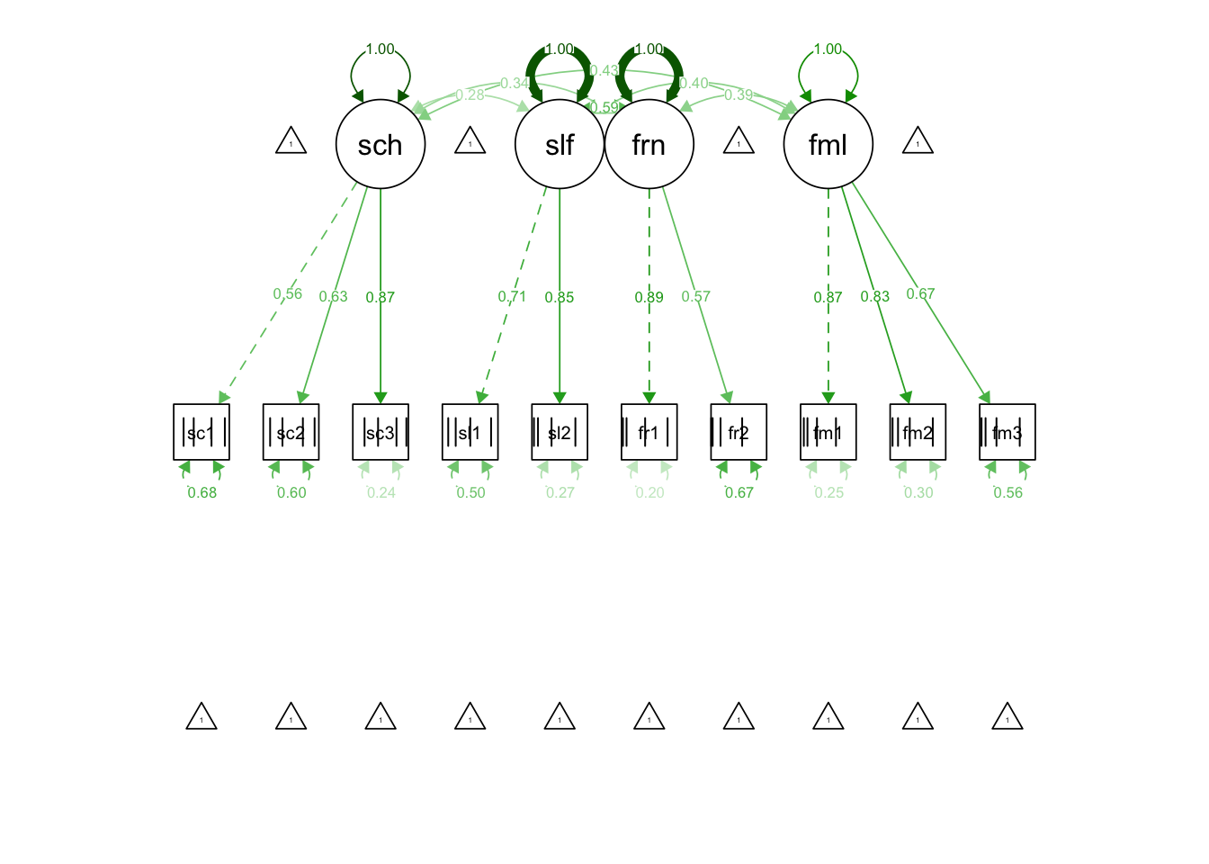
13.1.5 Life satisfaction CFA with three factors
Model definition
Since a prior PCA suggested that 3 factors might be enough we would like to check this model using a CFA approach. Thus, we define an additional model with only three factors (friends and self factors are combined). (Ideally, the PCA should not have been carried out on the same data.)
model_3f <- "
school =~ school1 + school2 + school3
self_friends =~ self1 + self2 + friends1 + friends2
family =~ fam1 + fam2 + fam3
"
Model estimation
fit_mod3f <- cfa(model_3f,
                 data = lifesat,
                 estimator = "MLM")
summary(fit_mod3f, fit.measures = TRUE, standardized = TRUE)
## lavaan 0.6-9 ended normally after 40 iterations
##
## Estimator ML
## Optimization method NLMINB
## Number of model parameters 23
##
## Number of observations 275
##
## Model Test User Model:
## Standard Robust
## Test Statistic 108.940 70.324
## Degrees of freedom 32 32
## P-value (Chi-square) 0.000 0.000
## Scaling correction factor 1.549
## Satorra-Bentler correction
##
## Model Test Baseline Model:
##
## Test statistic 725.606 420.551
## Degrees of freedom 45 45
## P-value 0.000 0.000
## Scaling correction factor 1.725
##
## User Model versus Baseline Model:
##
## Comparative Fit Index (CFI) 0.887 0.898
## Tucker-Lewis Index (TLI) 0.841 0.856
##
## Robust Comparative Fit Index (CFI) 0.908
## Robust Tucker-Lewis Index (TLI) 0.871
##
## Loglikelihood and Information Criteria:
##
## Loglikelihood user model (H0) -4085.347 -4085.347
## Loglikelihood unrestricted model (H1) -4030.877 -4030.877
##
## Akaike (AIC) 8216.694 8216.694
## Bayesian (BIC) 8299.880 8299.880
## Sample-size adjusted Bayesian (BIC) 8226.951 8226.951
##
## Root Mean Square Error of Approximation:
##
## RMSEA 0.094 0.066
## 90 Percent confidence interval - lower 0.075 0.049
## 90 Percent confidence interval - upper 0.113 0.083
## P-value RMSEA <= 0.05 0.000 0.058
##
## Robust RMSEA 0.082
## 90 Percent confidence interval - lower 0.056
## 90 Percent confidence interval - upper 0.108
##
## Standardized Root Mean Square Residual:
##
## SRMR 0.071 0.071
##
## Parameter Estimates:
##
## Standard errors Robust.sem
## Information Expected
## Information saturated (h1) model Structured
##
## Latent Variables:
## Estimate Std.Err z-value P(>|z|) Std.lv Std.all
## school =~
## school1 1.000 0.645 0.451
## school2 1.304 0.275 4.735 0.000 0.841 0.636
## school3 1.769 0.347 5.099 0.000 1.140 0.813
## self_friends =~
## self1 1.000 0.901 0.683
## self2 0.949 0.135 7.051 0.000 0.854 0.751
## friends1 0.600 0.149 4.031 0.000 0.540 0.530
## friends2 0.331 0.085 3.877 0.000 0.298 0.367
## family =~
## fam1 1.000 1.021 0.772
## fam2 1.041 0.150 6.958 0.000 1.063 0.867
## fam3 0.630 0.118 5.355 0.000 0.643 0.575
##
## Covariances:
## Estimate Std.Err z-value P(>|z|) Std.lv Std.all
## school ~~
## self_friends 0.177 0.065 2.718 0.007 0.304 0.304
## family 0.257 0.074 3.493 0.000 0.390 0.390
## self_friends ~~
## family 0.403 0.125 3.232 0.001 0.438 0.438
##
## Variances:
## Estimate Std.Err z-value P(>|z|) Std.lv Std.all
## .school1 1.627 0.175 9.270 0.000 1.627 0.796
## .school2 1.041 0.207 5.032 0.000 1.041 0.595
## .school3 0.669 0.270 2.479 0.013 0.669 0.340
## .self1 0.928 0.165 5.634 0.000 0.928 0.534
## .self2 0.564 0.160 3.527 0.000 0.564 0.436
## .friends1 0.748 0.110 6.771 0.000 0.748 0.719
## .friends2 0.572 0.056 10.142 0.000 0.572 0.866
## .fam1 0.706 0.153 4.619 0.000 0.706 0.404
## .fam2 0.373 0.121 3.069 0.002 0.373 0.248
## .fam3 0.838 0.120 6.961 0.000 0.838 0.669
## school 0.416 0.123 3.385 0.001 1.000 1.000
## self_friends 0.811 0.200 4.052 0.000 1.000 1.000
## family 1.043 0.231 4.508 0.000 1.000 1.000Global model fit
CFI = 0.908 and NNFI/TLI = 0.871 do not reach the recommended cut-off criteria. The RMSEA = 0.082 now is also significantly greater than 0.05 (90 %-CI [0.056; 0.108]).
Optional: Alternative definition of the 3-factor model
A 3-factor model can alternatively be specified by restricting certain parameters of the 4-factor model. This allows us to show that the 3-factor model is nested in the 4-factor model.
To turn the 4-factor model into a 3-factor model with a combined self-and-friends-factor, we have to make sure that the factors friends and self behave like a single factor using parameter restrictions.
For these two factors to become one, the covariance between the two factors must be set to 1 (see syntax below). For a covariance of 1 to really represent an exact equality of the two factors, the variances of the two latent variables must also be set to 1 (thus the correlation between the latent variables becomes 1). The easiest way to achieve this is to set the variances of all latent variables to the value 1 using the cfa() argument std.lv = TRUE, which at the same time ensures that the loadings of the first manifest variables of each factor are estimated freely. This aspect of the model is not defined in the model definition, but in the model estimation.
On the other hand, the relationships of the factors with all other factors must be identical for both factors (friends and self).
We can achieve this by naming (i.e. explicitly specifying) the parameters of the factor covariances and at the same time giving the same name to parameters to be equated. For example, the covariance of friends and school should be estimated exactly the same as the covariance between self and school. If we name both parameters with a, lavaan recognizes that the same value should be estimated for both covariances.
We call this model model_4f_res.
model_4f_res <- "
school =~ school1 + school2 + school3
self =~ self1 + self2
friends =~ friends1 + friends2
family =~ fam1 + fam2 + fam3

# Fixing the covariance to 1
friends ~~ 1*self

# Equality constraints: Covariances with equal parameter names
friends ~~ a*school
self ~~ a*school
friends ~~ b*family
self ~~ b*family
"
Estimating the alternative 3-factor model:
fit_mod4f_res <- cfa(model_4f_res,
                     std.lv = TRUE,
                    data = lifesat,
                 estimator = "MLM")

semPaths(fit_mod4f_res, "std")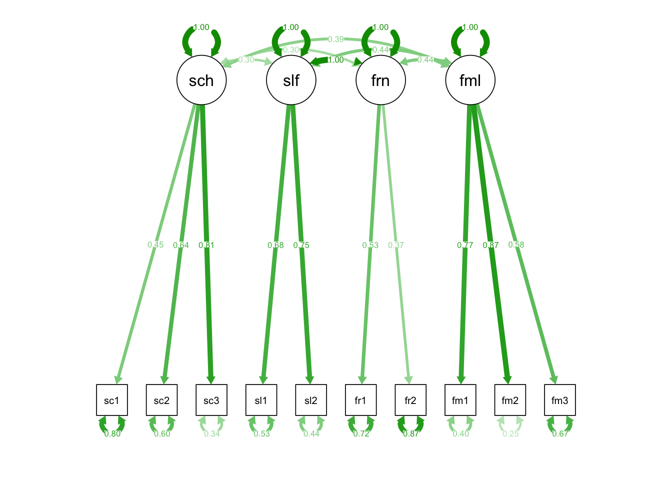
Model comparison of the 3-factor model and the alternative 3-factor model
A model comparison should now show that the 3-factor model and the restricted 4-factor model do have the same model fit, i.e. are identical:
anova(fit_mod3f, fit_mod4f_res)## Warning in lavTestLRT(object = object, ..., model.names = NAMES): lavaan
## WARNING: some models have the same degrees of freedom## Scaled Chi-Squared Difference Test (method = "satorra.bentler.2001")
##
## lavaan NOTE:
## The "Chisq" column contains standard test statistics, not the
## robust test that should be reported per model. A robust difference
## test is a function of two standard (not robust) statistics.
##
## Df AIC BIC Chisq Chisq diff Df diff Pr(>Chisq)
## fit_mod3f 32 8216.7 8299.9 108.94
## fit_mod4f_res 32 8216.7 8299.9 108.94 7.4448e-10 0Exactly! (The very small number at Chisq diff is caused by minimal numerical inaccuracies in the ML estimation.)
Model comparison of the 3-factor model and the 4-factor model
Now we want to test the 3-factor model against the original 4-factor model.
This test examines whether the null hypothesis that the 3-factor model does not fit worse to the data than the 4-factor model has to be rejected.
anova(fit_mod3f, fit_mod4f)## Scaled Chi-Squared Difference Test (method = "satorra.bentler.2001")
##
## lavaan NOTE:
## The "Chisq" column contains standard test statistics, not the
## robust test that should be reported per model. A robust difference
## test is a function of two standard (not robust) statistics.
##
## Df AIC BIC Chisq Chisq diff Df diff Pr(>Chisq)
## fit_mod4f 29 8182.0 8276.0 68.21
## fit_mod3f 32 8216.7 8299.9 108.94 16.324 3 0.000973 ***
## ---
## Signif. codes: 0 '***' 0.001 '**' 0.01 '*' 0.05 '.' 0.1 ' ' 1The comparison is significant. The 3-factor model therefore fits the data significantly worse than the 4-factor model.
For the AIC, a value of 8181.964 was obtained for the 4-factor model and a value of 8216.694 for the 3-factor model. Thus, the 4-factor model should be preferred (smaller AIC).
A similar picture emerges for the BIC: BIC = 8276 for the 4-factor model and BIC = 8299.88 for the 3-factor model. Thus, even according to the more parsimonious BIC (favors models with fewer parameters as compared to the AIC), the 4-factor model should be selected.
13.1.6 Model with a second order factor
As we can see, the factors in the 4-factor model are all positively correlated (and significantly so). This and the fact that life satisfaction in psychological research is conceptualized not only domain-specifically, but also (and even predominantly) globally, suggests that a 2nd order factor life satisfaction might exist. In other words: general life satisfaction factor might explain the inter-correlations among the domain-specific (first order) life satisfaction factors.
In CFA we can model such a second order factor. Another factor seems to make the model more complicated at first, but this can be misleading: In fact, in a model with one second order factor, there are two parameters less to be estimated than in a model with only four first order factors: Instead of six covariances among the factors, now four loadings (or three loadings and one second order factor variance) have to be estimated.
Model definition
model_4f_2order <-  "
school =~ school1 + school2 + school3
self =~ self1 + self2
friends =~ friends1 + friends2
family =~ fam1 + fam2 + fam3

# Second order factor life_satisfaction
life_satisfaction =~ school + self + friends + family
"
Model estimation
fit_mod4f_2order <- cfa(model_4f_2order,
                        data = lifesat,
                        estimator = "MLM")

semPaths(fit_mod4f_2order, "std")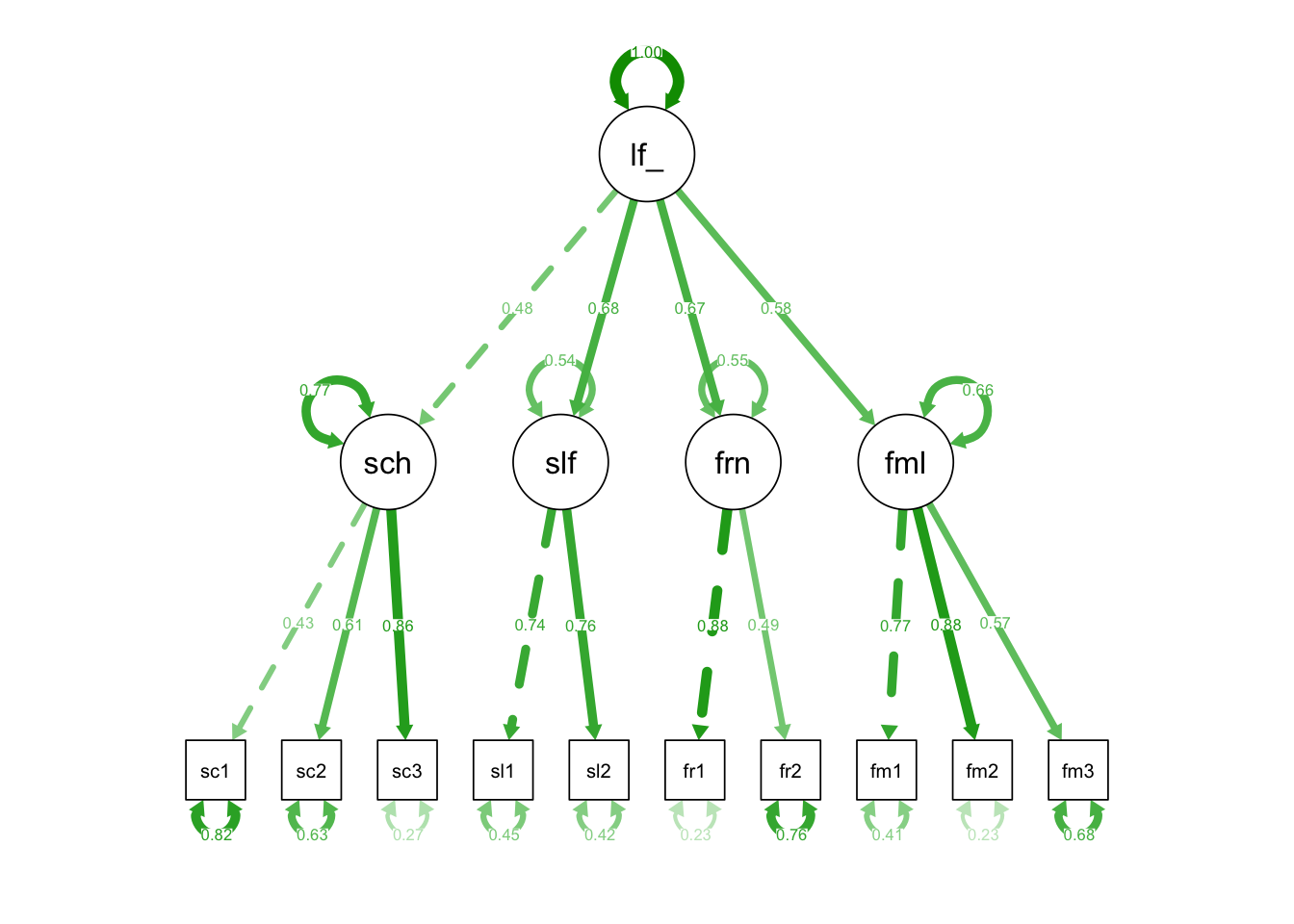
summary(fit_mod4f_2order, fit.measures = TRUE, standardized = TRUE)## lavaan 0.6-9 ended normally after 54 iterations
##
## Estimator ML
## Optimization method NLMINB
## Number of model parameters 24
##
## Number of observations 275
##
## Model Test User Model:
## Standard Robust
## Test Statistic 73.985 50.860
## Degrees of freedom 31 31
## P-value (Chi-square) 0.000 0.014
## Scaling correction factor 1.455
## Satorra-Bentler correction
##
## Model Test Baseline Model:
##
## Test statistic 725.606 420.551
## Degrees of freedom 45 45
## P-value 0.000 0.000
## Scaling correction factor 1.725
##
## User Model versus Baseline Model:
##
## Comparative Fit Index (CFI) 0.937 0.947
## Tucker-Lewis Index (TLI) 0.908 0.923
##
## Robust Comparative Fit Index (CFI) 0.955
## Robust Tucker-Lewis Index (TLI) 0.935
##
## Loglikelihood and Information Criteria:
##
## Loglikelihood user model (H0) -4067.870 -4067.870
## Loglikelihood unrestricted model (H1) -4030.877 -4030.877
##
## Akaike (AIC) 8183.739 8183.739
## Bayesian (BIC) 8270.542 8270.542
## Sample-size adjusted Bayesian (BIC) 8194.442 8194.442
##
## Root Mean Square Error of Approximation:
##
## RMSEA 0.071 0.048
## 90 Percent confidence interval - lower 0.050 0.027
## 90 Percent confidence interval - upper 0.092 0.068
## P-value RMSEA <= 0.05 0.048 0.534
##
## Robust RMSEA 0.058
## 90 Percent confidence interval - lower 0.027
## 90 Percent confidence interval - upper 0.086
##
## Standardized Root Mean Square Residual:
##
## SRMR 0.067 0.067
##
## Parameter Estimates:
##
## Standard errors Robust.sem
## Information Expected
## Information saturated (h1) model Structured
##
## Latent Variables:
## Estimate Std.Err z-value P(>|z|) Std.lv Std.all
## school =~
## school1 1.000 0.612 0.428
## school2 1.321 0.279 4.740 0.000 0.808 0.611
## school3 1.964 0.393 4.994 0.000 1.202 0.856
## self =~
## self1 1.000 0.978 0.741
## self2 0.886 0.147 6.022 0.000 0.866 0.761
## friends =~
## friends1 1.000 0.894 0.877
## friends2 0.445 0.155 2.869 0.004 0.398 0.490
## family =~
## fam1 1.000 1.014 0.767
## fam2 1.060 0.151 7.029 0.000 1.075 0.877
## fam3 0.628 0.115 5.444 0.000 0.637 0.569
## life_satisfaction =~
## school 1.000 0.480 0.480
## self 2.255 0.734 3.072 0.002 0.678 0.678
## friends 2.049 0.708 2.892 0.004 0.674 0.674
## family 2.011 0.680 2.959 0.003 0.583 0.583
##
## Variances:
## Estimate Std.Err z-value P(>|z|) Std.lv Std.all
## .school1 1.668 0.176 9.486 0.000 1.668 0.817
## .school2 1.094 0.204 5.358 0.000 1.094 0.626
## .school3 0.525 0.287 1.827 0.068 0.525 0.267
## .self1 0.783 0.180 4.345 0.000 0.783 0.450
## .self2 0.544 0.164 3.312 0.001 0.544 0.420
## .friends1 0.241 0.231 1.042 0.297 0.241 0.232
## .friends2 0.502 0.062 8.075 0.000 0.502 0.760
## .fam1 0.721 0.154 4.675 0.000 0.721 0.412
## .fam2 0.347 0.120 2.897 0.004 0.347 0.231
## .fam3 0.846 0.122 6.912 0.000 0.846 0.676
## .school 0.288 0.087 3.307 0.001 0.769 0.769
## .self 0.517 0.208 2.487 0.013 0.541 0.541
## .friends 0.436 0.240 1.816 0.069 0.546 0.546
## .family 0.679 0.182 3.725 0.000 0.660 0.660
## life_satisfctn 0.086 0.047 1.856 0.064 1.000 1.000The parameter estimates show that the strongest standardized loadings of the domain-specific (first order) factors are those of the self and of the friends factors, while the lowest is that of the school factor.
Model fit and model comparisons
Robust CFI = 0.955 and NNFI/TLI = 0.935 are very similar to the respective indices of the 4-factor model. The RMSEA = 0.058 is slightly lower than with the 4-factor model and not significantly greater than 0.05 (90 %-CI [0.027; 0.086]).
Now we compare all three models (in ascending order with regard to the number of estimated parameters: 3-factor model, 4-factor model with second-order factor, 4-factor model) using sequential likelihood-ratio tests. The prerequisite for the validity of these tests is the nesting of restricted models (with fewer parameters) in models with fewer restrictions (with more parameters). For the 3-factor and the 4-factor models we have demonstrated the nesting above. But also the 4-factor model with a second-order factor is nested in the 4-factor model (because actually all models that have the same four first order factors are nested in this model since it is a saturated model at the level of latent variables).
anova(fit_mod3f, fit_mod4f_2order, fit_mod4f)## Scaled Chi-Squared Difference Test (method = "satorra.bentler.2001")
##
## lavaan NOTE:
## The "Chisq" column contains standard test statistics, not the
## robust test that should be reported per model. A robust difference
## test is a function of two standard (not robust) statistics.
##
## Df AIC BIC Chisq Chisq diff Df diff Pr(>Chisq)
## fit_mod4f 29 8182.0 8276.0 68.210
## fit_mod4f_2order 31 8183.7 8270.5 73.985 3.8396 2 0.146639
## fit_mod3f 32 8216.7 8299.9 108.940 7.8078 1 0.005202 **
## ---
## Signif. codes: 0 '***' 0.001 '**' 0.01 '*' 0.05 '.' 0.1 ' ' 1The model comparison shows that the 4-factor model with a 2nd-order factor does not fit the data significantly worse than the less parsimonious 4-factor model (\(\Delta\chi^2=\) 3.8396, \(p =\) 0.1466). The second test, on the other hand, shows a significant model comparison of the 3-factor model with the 4-factor model with a second-order factor (\(\Delta\chi^2=\) 7.8078, \(p =\) 0.0052).
The best of these three models is therefore the 4-factor model with a 2nd-order factor. With regard to information criteria this model also has the lowest Bayesian Information Criterion (BIC = 8270.5 while the model with lowest Akaike Information Criterion (favoring less parsimonious models with more parameters) is the original 4-factor model (AIC = 8183.7).
13.2 Structural Equation Modelling (SEM)
13.2.1 Introduction
SEM represents a combination of CFA with regression models and allows to model complex regression structures (path models) at the level of latent variables. Indirect effects (mediation models) can also be estimated. The estimation theory does not differ from that of CFA.
As an example we will study the effects of emotional support by parents and friends as experienced by adolescents on their life satisfaction. The two self-efficacy domains “academic self-efficacy” and “social self-efficacy” will serve as mediators for these effects. Both direct and indirect effects will be investigated.
Theoretical basis and hypotheses: Both parental support and support from friends have a positive effect on life satisfaction. In addition, it is known from self-efficacy research that experienced support can have positive effects on the experience of self-efficacy, and that this experience in turn is related to higher life satisfaction. An important question, however, concerns the differential effects resulting when these constructs with their respective domains are considered simultaneously.
The assumed effects can be summarized in the following structural model:

For the postulated structural model (relations between the latent variables) we need a measurement model (relations between the latent variables and the manifest variables, i.e. the factor structure). With a large number of measured variables the measurement model is often based on “packages” of individual items rather than on the individual items themselves. Here we choose the “item-to-construct balance approach” to packaging (Little et al., 2002), in which individual items representing a certain construct are combined in such a way that the “packed” manifest variables load as homogeneously as possible on the respective latent factor. It is generally recommended to use three to four parcels per latent variable.
The following parcels were built:
Emotional support from parents (6 items): 3 parcels of 2 items (sup_parents_p1, sup_parents_p2, sup_parents_p3)
Emotional support from friends (6 items): 3 parcels of 2 items (sup_friends_p1, sup_friends_p2, sup_friends_p3)
Academic self-efficacy (20 items): 2 parcels of 7 items & 1 parcel of 6 items (se_acad_p1, se_acad_p2, se_acad_p3)
Social self-efficacy (16 items): 2 parcels of 5 items & 1 parcel of 6 items (se_social_p1, se_social_p2, se_social_p3)
Life satisfaction (11 items): 2 parcels of 4 items & 1 parcel of 3 items (ls_p1, ls_p2, ls_p3)
The SEM analysis is carried out in three steps:
We start with the measurement model. The measurement model is a multi-construct CFA with intercorrelations of all latent variables.
Then we consider the entire structural equation model (measurement and structural model combined).
In the last step we will show how to explicitly define indirect and total effects within the SEM.
13.2.2 Importing the data
data_sem <- read_csv(
  url("https://raw.githubusercontent.com/methodenlehre/data/master/sem_data.csv"))
## Rows: 283 Columns: 19## ── Column specification ────────────────────────────────────────────────────────
## Delimiter: ","
## chr (2): region, gender
## dbl (17): ID, age, se_acad_p1, se_acad_p2, se_acad_p3, se_social_p1, se_soci...##
## ℹ Use `spec()` to retrieve the full column specification for this data.
## ℹ Specify the column types or set `show_col_types = FALSE` to quiet this message.# convert ID and gender to factors
data_sem$ID <- as.factor(data_sem$ID)
data_sem$region <- as.factor(data_sem$region)
data_sem$gender <- as.factor(data_sem$gender)13.2.3 Measurement model
In the measurement model, the relationships between the latent variables (factors) and the manifest variables are defined. We are already familiar with the lavaan model definition from the CFA example above.
Error variances of the observed variables and variances of the exogenous latent variables do not have to be explicitly specified.
Operator for the measuring model:
=~(“is measured by…”)
model_measurement <- "
# Measurement model
SUP_Parents =~ sup_parents_p1 + sup_parents_p2 + sup_parents_p3
SUP_Friends =~ sup_friends_p1 + sup_friends_p2 + sup_friends_p3
SE_Academic =~ se_acad_p1 + se_acad_p2 + se_acad_p3
SE_Social =~ se_social_p1 + se_social_p2 + se_social_p3
LS  =~ ls_p1 + ls_p2 + ls_p3
"
Model estimation
The function sem() is applied to the model_measurement specified above, and the results are stored in an object (here fit_measurement). We could also use cfa() here. The two functions differ only slightly in their default settings and are both equally suitable for estimating measurement models.
Let’s have a look at univariate and multivariate normality of the data:
# univariate skewness and kurtosis
check_sem <- data_sem[-(1:4)] %>%
  describe()

check_sem$skew
## [1] -0.2629296 -0.3354220 -0.2959812 -0.5640013 -0.6063687 -0.4473382
## [7] -1.2294259 -1.2473578 -1.5262892 -1.4238442 -1.1944909 -1.2408782
## [13] -0.7683010 -1.2142986 -0.6984612check_sem$kurtosis## [1] -0.4082208 -0.2082133 -0.1383948 1.4428096 0.7746075 -0.1695429
## [7] 1.8438486 1.6086578 2.7745329 2.6667347 1.1928812 1.7737603
## [13] 0.7185157 2.8794007 0.5447682# multivariate skewness and kurtosis
data_sem[-(1:4)] %>%
mardiaSkew()## b1d chi df p
## 4.617123e+01 2.177743e+03 6.800000e+02 4.263531e-156data_sem[-(1:4)] %>%
mardiaKurtosis()## b2d z p
## 3.328664e+02 2.900204e+01 6.201873e-185fit_measurement <- sem(model_measurement,
data = data_sem,
estimator = "MLM")
summary(fit_measurement, fit.measures = TRUE, standardized = TRUE)## lavaan 0.6-9 ended normally after 49 iterations
##
## Estimator ML
## Optimization method NLMINB
## Number of model parameters 40
##
## Number of observations 283
##
## Model Test User Model:
## Standard Robust
## Test Statistic 223.992 183.847
## Degrees of freedom 80 80
## P-value (Chi-square) 0.000 0.000
## Scaling correction factor 1.218
## Satorra-Bentler correction
##
## Model Test Baseline Model:
##
## Test statistic 2696.489 1983.449
## Degrees of freedom 105 105
## P-value 0.000 0.000
## Scaling correction factor 1.359
##
## User Model versus Baseline Model:
##
## Comparative Fit Index (CFI) 0.944 0.945
## Tucker-Lewis Index (TLI) 0.927 0.927
##
## Robust Comparative Fit Index (CFI) 0.950
## Robust Tucker-Lewis Index (TLI) 0.935
##
## Loglikelihood and Information Criteria:
##
## Loglikelihood user model (H0) -4285.972 -4285.972
## Loglikelihood unrestricted model (H1) -4173.976 -4173.976
##
## Akaike (AIC) 8651.944 8651.944
## Bayesian (BIC) 8797.761 8797.761
## Sample-size adjusted Bayesian (BIC) 8670.921 8670.921
##
## Root Mean Square Error of Approximation:
##
## RMSEA 0.080 0.068
## 90 Percent confidence interval - lower 0.067 0.056
## 90 Percent confidence interval - upper 0.092 0.079
## P-value RMSEA <= 0.05 0.000 0.007
##
## Robust RMSEA 0.075
## 90 Percent confidence interval - lower 0.061
## 90 Percent confidence interval - upper 0.089
##
## Standardized Root Mean Square Residual:
##
## SRMR 0.056 0.056
##
## Parameter Estimates:
##
## Standard errors Robust.sem
## Information Expected
## Information saturated (h1) model Structured
##
## Latent Variables:
## Estimate Std.Err z-value P(>|z|) Std.lv Std.all
## SUP_Parents =~
## sup_parents_p1 1.000 0.935 0.873
## sup_parents_p2 1.036 0.061 16.969 0.000 0.969 0.887
## sup_parents_p3 0.996 0.070 14.274 0.000 0.932 0.816
## SUP_Friends =~
## sup_friends_p1 1.000 1.021 0.906
## sup_friends_p2 0.792 0.061 12.917 0.000 0.809 0.857
## sup_friends_p3 0.891 0.077 11.631 0.000 0.910 0.831
## SE_Academic =~
## se_acad_p1 1.000 0.695 0.878
## se_acad_p2 0.809 0.045 17.983 0.000 0.562 0.820
## se_acad_p3 0.955 0.057 16.681 0.000 0.664 0.829
## SE_Social =~
## se_social_p1 1.000 0.638 0.843
## se_social_p2 0.967 0.065 14.840 0.000 0.617 0.885
## se_social_p3 0.928 0.066 13.974 0.000 0.592 0.741
## LS =~
## ls_p1 1.000 0.667 0.718
## ls_p2 0.778 0.075 10.411 0.000 0.519 0.712
## ls_p3 0.968 0.086 11.272 0.000 0.645 0.732
##
## Covariances:
## Estimate Std.Err z-value P(>|z|) Std.lv Std.all
## SUP_Parents ~~
## SUP_Friends 0.132 0.066 2.012 0.044 0.138 0.138
## SE_Academic 0.218 0.043 5.071 0.000 0.336 0.336
## SE_Social 0.282 0.063 4.457 0.000 0.472 0.472
## LS 0.405 0.065 6.275 0.000 0.650 0.650
## SUP_Friends ~~
## SE_Academic 0.071 0.044 1.611 0.107 0.100 0.100
## SE_Social 0.196 0.039 5.057 0.000 0.301 0.301
## LS 0.175 0.050 3.482 0.000 0.257 0.257
## SE_Academic ~~
## SE_Social 0.271 0.035 7.665 0.000 0.611 0.611
## LS 0.238 0.043 5.496 0.000 0.514 0.514
## SE_Social ~~
## LS 0.321 0.053 6.004 0.000 0.755 0.755
##
## Variances:
## Estimate Std.Err z-value P(>|z|) Std.lv Std.all
## .sup_parents_p1 0.273 0.043 6.355 0.000 0.273 0.238
## .sup_parents_p2 0.255 0.054 4.717 0.000 0.255 0.213
## .sup_parents_p3 0.437 0.070 6.280 0.000 0.437 0.335
## .sup_friends_p1 0.227 0.071 3.186 0.001 0.227 0.179
## .sup_friends_p2 0.238 0.054 4.408 0.000 0.238 0.266
## .sup_friends_p3 0.371 0.097 3.832 0.000 0.371 0.310
## .se_acad_p1 0.144 0.028 5.149 0.000 0.144 0.229
## .se_acad_p2 0.153 0.020 7.629 0.000 0.153 0.327
## .se_acad_p3 0.200 0.031 6.547 0.000 0.200 0.313
## .se_social_p1 0.166 0.023 7.060 0.000 0.166 0.290
## .se_social_p2 0.106 0.017 6.150 0.000 0.106 0.217
## .se_social_p3 0.288 0.028 10.373 0.000 0.288 0.451
## .ls_p1 0.417 0.048 8.643 0.000 0.417 0.484
## .ls_p2 0.261 0.057 4.568 0.000 0.261 0.492
## .ls_p3 0.362 0.046 7.942 0.000 0.362 0.465
## SUP_Parents 0.875 0.147 5.958 0.000 1.000 1.000
## SUP_Friends 1.042 0.148 7.025 0.000 1.000 1.000
## SE_Academic 0.483 0.049 9.919 0.000 1.000 1.000
## SE_Social 0.407 0.062 6.518 0.000 1.000 1.000
## LS 0.444 0.076 5.826 0.000 1.000 1.000As can be seen from the output the standardized loadings are all relatively high and also homogeneous. The factor correlations of this multi-construct measurement model are between \(r = 0.100\) (SUP_Friends \(\leftrightarrow\) SE_Academic) and \(r = 0.755\) (SE_Social \(\leftrightarrow\) LS).
Global model fit is not really good (CFI = 0.95, NNFI/TLI = 0.935, RMSEA = 0.075, 90 %-CI: [0.061; 0.089]) but can still be seen as acceptable according to commonly accepted criteria.
In order to determine where problems exist in the model fit, we can first consider the standardized residual variance-covariance matrix:
resid(fit_measurement, type = "standardized")$cov## sp_p_1 sp_p_2 sp_p_3 sp_f_1 sp_f_2 sp_f_3 s_cd_1 s_cd_2 s_cd_3
## sup_parents_p1 0.000
## sup_parents_p2 2.434 0.000
## sup_parents_p3 -1.429 -1.067 0.000
## sup_friends_p1 0.866 1.006 -3.755 0.000
## sup_friends_p2 1.269 1.365 -1.737 0.872 0.000
## sup_friends_p3 0.636 1.022 -2.149 0.695 -1.351 0.000
## se_acad_p1 -0.622 -1.488 2.267 -0.629 0.066 0.719 0.000
## se_acad_p2 -0.561 -0.644 1.500 0.636 0.925 0.464 -0.776 0.000
## se_acad_p3 -0.724 -0.930 2.396 -1.726 0.299 -0.128 0.421 0.250 0.000
## se_social_p1 1.369 0.658 2.131 -3.995 -1.830 -1.750 3.100 0.822 1.063
## se_social_p2 -0.168 -0.606 -0.251 1.021 1.738 1.662 -1.766 -0.652 -2.323
## se_social_p3 -1.332 -1.108 -0.929 2.452 0.429 1.255 -0.144 1.448 -0.624
## ls_p1 -2.573 -3.037 0.431 -3.825 -1.256 -1.387 -0.667 2.059 1.091
## ls_p2 -1.485 -2.864 -0.651 2.180 4.373 3.112 -2.427 -1.568 -2.791
## ls_p3 2.056 3.067 4.537 -1.555 -0.217 -0.289 1.661 1.410 1.896
## s_sc_1 s_sc_2 s_sc_3 ls_p1 ls_p2 ls_p3
## sup_parents_p1
## sup_parents_p2
## sup_parents_p3
## sup_friends_p1
## sup_friends_p2
## sup_friends_p3
## se_acad_p1
## se_acad_p2
## se_acad_p3
## se_social_p1 0.000
## se_social_p2 0.786 0.000
## se_social_p3 -2.264 1.130 0.000
## ls_p1 -0.391 -0.899 -0.384 0.000
## ls_p2 2.483 1.884 2.431 2.206 0.000
## ls_p3 -1.080 -2.168 -1.795 0.956 -3.811 0.000This shows that the variance-covariance matrix implied by the model deviates significantly from the empirical variance-covariance matrix for a number of covariances, e.g. for sp_p_3 ~~ ls_p3 or for sp_f_2 ~~ ls_p2.
Modification indices
Another possibility for local fit diagnostics is offered by modification indices. These indicate which additional model parameters would result in a significant fit improvement (in terms of a reduction of \(\chi^2\) by the value of the corresponding MI). We will only display the MI \(\geq 5\), since usually only those are considered substantial.
modindices(fit_measurement, standardized = FALSE, minimum.value = 5)## lhs op rhs mi epc
## 55 SUP_Parents =~ ls_p1 8.480 -0.237
## 56 SUP_Parents =~ ls_p2 6.169 -0.158
## 57 SUP_Parents =~ ls_p3 28.086 0.411
## 60 SUP_Friends =~ sup_parents_p3 16.443 -0.189
## 64 SUP_Friends =~ se_social_p1 16.789 -0.134
## 65 SUP_Friends =~ se_social_p2 5.289 0.069
## 67 SUP_Friends =~ ls_p1 6.881 -0.133
## 68 SUP_Friends =~ ls_p2 15.119 0.155
## 72 SE_Academic =~ sup_parents_p3 8.733 0.218
## 76 SE_Academic =~ se_social_p1 9.991 0.206
## 77 SE_Academic =~ se_social_p2 9.885 -0.190
## 80 SE_Academic =~ ls_p2 11.947 -0.247
## 81 SE_Academic =~ ls_p3 5.984 0.212
## 92 SE_Social =~ ls_p2 12.281 0.440
## 93 SE_Social =~ ls_p3 6.535 -0.393
## 96 LS =~ sup_parents_p3 6.743 0.286
## 106 sup_parents_p1 ~~ sup_parents_p2 9.237 0.196
## 133 sup_parents_p3 ~~ sup_friends_p1 9.338 -0.084
## 144 sup_parents_p3 ~~ ls_p3 9.302 0.090
## 150 sup_friends_p1 ~~ se_social_p1 8.932 -0.053
## 152 sup_friends_p1 ~~ se_social_p3 18.792 0.094
## 162 sup_friends_p2 ~~ se_social_p3 8.353 -0.056
## 164 sup_friends_p2 ~~ ls_p2 5.784 0.046
## 177 se_acad_p1 ~~ se_social_p1 12.065 0.047
## 180 se_acad_p1 ~~ ls_p1 6.839 -0.053
## 187 se_acad_p2 ~~ ls_p1 5.411 0.044
## 194 se_acad_p3 ~~ ls_p2 5.268 -0.040
## 197 se_social_p1 ~~ se_social_p3 5.022 -0.046
## 206 se_social_p3 ~~ ls_p2 9.322 0.059
## 208 ls_p1 ~~ ls_p2 7.056 0.079
## 210 ls_p2 ~~ ls_p3 13.346 -0.105A total of 31 modification indices are displayed. They refer either to possible cross-loadings (e.g. SUP_Parents =~ ls_p3: MI = 28.086) or to residual covariances between manifest variables (e.g. sup_friends_p1 ~~ se_social_p3: MI = 18.792). For theoretical reasons it is not recommended to add cross-loadings or residual covariances (especially across different latent variables) to the model.
Such model fit problems often arise in self-report studies. Individual differences in scale use (response styles) can play a role: These can lead to generally increased correlations among the variables, which may not be adequately taken into account in a multi-construct measurement model. There are approaches (definition of method and response style factors) to deal with this issue.
Another reason for the model-fit problems in this study could be the general similarity of the constructs investigated with respect to life domains. For example, there are life satisfaction items with respect to friends, but the friends context also plays an important role for the items for social self-efficacy and, of course, for support received from friends.
Since the model fit is still acceptable, we continue to work with this measurement model. In the next step we will model the effects among latent variables in order to test our theoretical assumptions (structural model).
13.2.4 Structural model
Model definition
The structural model represents the relationships/effects among the latent variables. It is added to the measurement model definitions:
model <- "
# Measurement model
SUP_Parents =~ sup_parents_p1 + sup_parents_p2 + sup_parents_p3
SUP_Friends =~ sup_friends_p1 + sup_friends_p2 + sup_friends_p3
SE_Academic =~ se_acad_p1 + se_acad_p2 + se_acad_p3
SE_Social =~ se_social_p1 + se_social_p2 + se_social_p3
LS  =~ ls_p1 + ls_p2 + ls_p3

# Structural model
# Regressions
SE_Academic ~ SUP_Parents + SUP_Friends
SE_Social ~ SUP_Parents + SUP_Friends
LS ~ SE_Academic + SE_Social + SUP_Parents + SUP_Friends

# Residual covariances
SE_Academic ~~ SE_Social
"
Operator for the structural model (regressions of latent variables):
~(“is predicted by…”)Operator for (residual) variances and covariances:
~~(for variances, the same variable appears on the left and right; for covariances, different variables). As in the measurement model (CFA), variances and covariances of exogenous latent variables do not have to be specified (are automatically estimated). The residual variances of endogenous latent variables are also estimated automatically.
Therefore we only have to specify one parameter using ~~: In this model we have two parallel latent mediator variables (SE_Academic and SE_Social) which have no effects on each other. However, it can be assumed that these two variables (or rather their residuals) co-vary since a general self-efficacy component is likely (cf. also the correlation of \(r=0.621\) in the measurement model above). Since SE_Academic and SE_Social are endogenous latent variables (both are predicted by both SUP_Parents and SUP_Friends), a residual covariance \(\psi =\) SE_Academic ~~ SE_Social must be specified.
Model estimation
fit <- sem(model,
           data = data_sem,
           estimator = "MLM")
summary(fit, fit.measures = TRUE, standardized = TRUE)
## lavaan 0.6-9 ended normally after 43 iterations
##
## Estimator ML
## Optimization method NLMINB
## Number of model parameters 40
##
## Number of observations 283
##
## Model Test User Model:
## Standard Robust
## Test Statistic 223.992 183.847
## Degrees of freedom 80 80
## P-value (Chi-square) 0.000 0.000
## Scaling correction factor 1.218
## Satorra-Bentler correction
##
## Model Test Baseline Model:
##
## Test statistic 2696.489 1983.449
## Degrees of freedom 105 105
## P-value 0.000 0.000
## Scaling correction factor 1.359
##
## User Model versus Baseline Model:
##
## Comparative Fit Index (CFI) 0.944 0.945
## Tucker-Lewis Index (TLI) 0.927 0.927
##
## Robust Comparative Fit Index (CFI) 0.950
## Robust Tucker-Lewis Index (TLI) 0.935
##
## Loglikelihood and Information Criteria:
##
## Loglikelihood user model (H0) -4285.972 -4285.972
## Loglikelihood unrestricted model (H1) -4173.976 -4173.976
##
## Akaike (AIC) 8651.944 8651.944
## Bayesian (BIC) 8797.761 8797.761
## Sample-size adjusted Bayesian (BIC) 8670.921 8670.921
##
## Root Mean Square Error of Approximation:
##
## RMSEA 0.080 0.068
## 90 Percent confidence interval - lower 0.067 0.056
## 90 Percent confidence interval - upper 0.092 0.079
## P-value RMSEA <= 0.05 0.000 0.007
##
## Robust RMSEA 0.075
## 90 Percent confidence interval - lower 0.061
## 90 Percent confidence interval - upper 0.089
##
## Standardized Root Mean Square Residual:
##
## SRMR 0.056 0.056
##
## Parameter Estimates:
##
## Standard errors Robust.sem
## Information Expected
## Information saturated (h1) model Structured
##
## Latent Variables:
## Estimate Std.Err z-value P(>|z|) Std.lv Std.all
## SUP_Parents =~
## sup_parents_p1 1.000 0.935 0.873
## sup_parents_p2 1.036 0.061 16.969 0.000 0.969 0.887
## sup_parents_p3 0.996 0.070 14.274 0.000 0.932 0.816
## SUP_Friends =~
## sup_friends_p1 1.000 1.021 0.906
## sup_friends_p2 0.792 0.061 12.917 0.000 0.809 0.857
## sup_friends_p3 0.891 0.077 11.631 0.000 0.910 0.831
## SE_Academic =~
## se_acad_p1 1.000 0.695 0.878
## se_acad_p2 0.809 0.045 17.983 0.000 0.562 0.820
## se_acad_p3 0.955 0.057 16.681 0.000 0.664 0.829
## SE_Social =~
## se_social_p1 1.000 0.638 0.843
## se_social_p2 0.967 0.065 14.840 0.000 0.617 0.885
## se_social_p3 0.928 0.066 13.974 0.000 0.592 0.741
## LS =~
## ls_p1 1.000 0.667 0.718
## ls_p2 0.778 0.075 10.411 0.000 0.519 0.712
## ls_p3 0.968 0.086 11.272 0.000 0.645 0.732
##
## Regressions:
## Estimate Std.Err z-value P(>|z|) Std.lv Std.all
## SE_Academic ~
## SUP_Parents 0.244 0.055 4.450 0.000 0.328 0.328
## SUP_Friends 0.037 0.044 0.843 0.399 0.054 0.054
## SE_Social ~
## SUP_Parents 0.300 0.062 4.850 0.000 0.439 0.439
## SUP_Friends 0.150 0.038 3.978 0.000 0.240 0.240
## LS ~
## SE_Academic 0.058 0.078 0.745 0.457 0.061 0.061
## SE_Social 0.553 0.091 6.081 0.000 0.529 0.529
## SUP_Parents 0.267 0.049 5.424 0.000 0.375 0.375
## SUP_Friends 0.026 0.036 0.727 0.467 0.040 0.040
##
## Covariances:
## Estimate Std.Err z-value P(>|z|) Std.lv Std.all
## .SE_Academic ~~
## .SE_Social 0.195 0.028 7.064 0.000 0.551 0.551
## SUP_Parents ~~
## SUP_Friends 0.132 0.066 2.012 0.044 0.138 0.138
##
## Variances:
## Estimate Std.Err z-value P(>|z|) Std.lv Std.all
## .sup_parents_p1 0.273 0.043 6.355 0.000 0.273 0.238
## .sup_parents_p2 0.255 0.054 4.717 0.000 0.255 0.213
## .sup_parents_p3 0.437 0.070 6.280 0.000 0.437 0.335
## .sup_friends_p1 0.227 0.071 3.186 0.001 0.227 0.179
## .sup_friends_p2 0.238 0.054 4.408 0.000 0.238 0.266
## .sup_friends_p3 0.371 0.097 3.832 0.000 0.371 0.310
## .se_acad_p1 0.144 0.028 5.149 0.000 0.144 0.229
## .se_acad_p2 0.153 0.020 7.629 0.000 0.153 0.327
## .se_acad_p3 0.200 0.031 6.547 0.000 0.200 0.313
## .se_social_p1 0.166 0.023 7.060 0.000 0.166 0.290
## .se_social_p2 0.106 0.017 6.150 0.000 0.106 0.217
## .se_social_p3 0.288 0.028 10.373 0.000 0.288 0.451
## .ls_p1 0.417 0.048 8.643 0.000 0.417 0.484
## .ls_p2 0.261 0.057 4.568 0.000 0.261 0.492
## .ls_p3 0.362 0.046 7.942 0.000 0.362 0.465
## SUP_Parents 0.875 0.147 5.958 0.000 1.000 1.000
## SUP_Friends 1.042 0.148 7.025 0.000 1.000 1.000
## .SE_Academic 0.427 0.043 9.863 0.000 0.884 0.884
## .SE_Social 0.293 0.041 7.200 0.000 0.720 0.720
## .LS 0.140 0.033 4.277 0.000 0.315 0.315The model fit is exactly the same! We have already seen above that we have just as many parameters and degrees of freedom in the overall model as in the measurement model.
This means that the structural model is saturated!
In the measurement model we had 15 variance and covariance parameters of the latent variables, so the variance-covariance matrix of the latent variables (with 5 x 6/2 = 15 elements) was complete and unrestricted. We now also have 15 parameters in the structural model. The parameters of the structural model are estimable and we can thus test our postulated effects, but this part of the overall model is just identified (since \(n_{Info} = n_{Par}\) with regard to the latent variables) and thus does not contribute to the model fit of the overall model! In other words: We cannot check whether the structural model fits our data well, only the fit of the measurement model can be tested.
Interpretation of the estimated structural coefficients:
Of the 8 postulated structural paths, 5 are significant and go in the expected direction. Not significant are the effects of SUP_Friends on SE_Academic (Std.all \(= 0.054,\ p = 0.399\)), from SE_Academic to LS (Std.all \(= 0.061,\ p = 0.457\)), and from SUP_Friends to LS (Std.all \(= 0.040,\ p = 0.467\)).
It is particularly striking that the perceived support by the parents has a substantial direct effect on life satisfaction, whereas the direct effect of the perceived support by the friends is not significant. It is also interesting that the academic self-efficacy no longer has a significant effect on satisfaction when social self-efficacy is held constant, even though the correlation between the two latent variables SE_Academic and LS was substantial in the measurement model (see above \(r = 0.514,\ p < 0.001\)).
Estimating indirect and total effects
With one or more latent mediator variables present in the structural model the SEM turns into a latent mediation analysis. To estimate indirect and total effects, the parameters of the structural model must first be explicitly named in the model definition (multiplication of predictors with b1, b2, b3, etc.).
Specific and total indirect effects can then be defined as products (or sum of products) of the path parameters (operator:
:=)Total effects can be defined equally as the sum of indirect and direct effects
When indirect and total effects are defined the model should always be estimated using the se = "bootstrap" option (even if the data are otherwise normally distributed). This is because other than the path coefficients themselves indirect effects (products of path coefficients) are not asymptotically normally distributed which renders the z- or Wald-approximation inappropriate for these defined parameters.
model_mediation <- '
# Measurement model
SUP_Parents =~ sup_parents_p1 + sup_parents_p2 + sup_parents_p3
SUP_Friends =~ sup_friends_p1 + sup_friends_p2 + sup_friends_p3
SE_Academic =~ se_acad_p1 + se_acad_p2 + se_acad_p3
SE_Social =~ se_social_p1 + se_social_p2 + se_social_p3
LS  =~ ls_p1 + ls_p2 + ls_p3

# Structural model
# Regressions
SE_Academic ~ b1*SUP_Parents + b3*SUP_Friends
SE_Social ~ b2*SUP_Parents + b4*SUP_Friends
LS ~ b5*SUP_Parents + b6*SUP_Friends + b7*SE_Academic + b8*SE_Social

# Residual covariances
SE_Academic ~~ SE_Social

# Indirect effects
b1b7 := b1*b7
b2b8 := b2*b8
totalind_eltern := b1*b7 + b2*b8
b3b7 := b3*b7
b4b8 := b4*b8
totalind_freunde := b3*b7 + b4*b8

# Total effects
total_eltern := b1*b7 + b2*b8 + b5
total_freunde := b3*b7 + b4*b8 + b6
'

fit_mediation <- sem(model_mediation,
                     data = data_sem,
                     se = "bootstrap",
                     verbose = FALSE,
                     bootstrap = 1000)
summary(fit_mediation, fit.measures = TRUE, standardized = TRUE)
## lavaan 0.6-9 ended normally after 43 iterations
##
## Estimator ML
## Optimization method NLMINB
## Number of model parameters 40
##
## Number of observations 283
##
## Model Test User Model:
##
## Test statistic 223.992
## Degrees of freedom 80
## P-value (Chi-square) 0.000
##
## Model Test Baseline Model:
##
## Test statistic 2696.489
## Degrees of freedom 105
## P-value 0.000
##
## User Model versus Baseline Model:
##
## Comparative Fit Index (CFI) 0.944
## Tucker-Lewis Index (TLI) 0.927
##
## Loglikelihood and Information Criteria:
##
## Loglikelihood user model (H0) -4285.972
## Loglikelihood unrestricted model (H1) -4173.976
##
## Akaike (AIC) 8651.944
## Bayesian (BIC) 8797.761
## Sample-size adjusted Bayesian (BIC) 8670.921
##
## Root Mean Square Error of Approximation:
##
## RMSEA 0.080
## 90 Percent confidence interval - lower 0.067
## 90 Percent confidence interval - upper 0.092
## P-value RMSEA <= 0.05 0.000
##
## Standardized Root Mean Square Residual:
##
## SRMR 0.056
##
## Parameter Estimates:
##
## Standard errors Bootstrap
## Number of requested bootstrap draws 1000
## Number of successful bootstrap draws 1000
##
## Latent Variables:
## Estimate Std.Err z-value P(>|z|) Std.lv Std.all
## SUP_Parents =~
## sup_parents_p1 1.000 0.935 0.873
## sup_parents_p2 1.036 0.062 16.817 0.000 0.969 0.887
## sup_parents_p3 0.996 0.076 13.073 0.000 0.932 0.816
## SUP_Friends =~
## sup_friends_p1 1.000 1.021 0.906
## sup_friends_p2 0.792 0.061 12.913 0.000 0.809 0.857
## sup_friends_p3 0.891 0.075 11.921 0.000 0.910 0.831
## SE_Academic =~
## se_acad_p1 1.000 0.695 0.878
## se_acad_p2 0.809 0.047 17.232 0.000 0.562 0.820
## se_acad_p3 0.955 0.056 16.948 0.000 0.664 0.829
## SE_Social =~
## se_social_p1 1.000 0.638 0.843
## se_social_p2 0.967 0.068 14.174 0.000 0.617 0.885
## se_social_p3 0.928 0.078 11.937 0.000 0.592 0.741
## LS =~
## ls_p1 1.000 0.667 0.718
## ls_p2 0.778 0.090 8.604 0.000 0.519 0.712
## ls_p3 0.968 0.103 9.434 0.000 0.645 0.732
##
## Regressions:
## Estimate Std.Err z-value P(>|z|) Std.lv Std.all
## SE_Academic ~
## SUP_Prnts (b1) 0.244 0.060 4.080 0.000 0.328 0.328
## SUP_Frnds (b3) 0.037 0.044 0.839 0.402 0.054 0.054
## SE_Social ~
## SUP_Prnts (b2) 0.300 0.063 4.776 0.000 0.439 0.439
## SUP_Frnds (b4) 0.150 0.039 3.797 0.000 0.240 0.240
## LS ~
## SUP_Prnts (b5) 0.267 0.058 4.579 0.000 0.375 0.375
## SUP_Frnds (b6) 0.026 0.042 0.634 0.526 0.040 0.040
## SE_Acadmc (b7) 0.058 0.099 0.589 0.556 0.061 0.061
## SE_Social (b8) 0.553 0.118 4.663 0.000 0.529 0.529
##
## Covariances:
## Estimate Std.Err z-value P(>|z|) Std.lv Std.all
## .SE_Academic ~~
## .SE_Social 0.195 0.029 6.653 0.000 0.551 0.551
## SUP_Parents ~~
## SUP_Friends 0.132 0.068 1.934 0.053 0.138 0.138
##
## Variances:
## Estimate Std.Err z-value P(>|z|) Std.lv Std.all
## .sup_parents_p1 0.273 0.040 6.757 0.000 0.273 0.238
## .sup_parents_p2 0.255 0.051 4.959 0.000 0.255 0.213
## .sup_parents_p3 0.437 0.071 6.151 0.000 0.437 0.335
## .sup_friends_p1 0.227 0.069 3.280 0.001 0.227 0.179
## .sup_friends_p2 0.238 0.052 4.577 0.000 0.238 0.266
## .sup_friends_p3 0.371 0.093 3.990 0.000 0.371 0.310
## .se_acad_p1 0.144 0.027 5.264 0.000 0.144 0.229
## .se_acad_p2 0.153 0.020 7.576 0.000 0.153 0.327
## .se_acad_p3 0.200 0.030 6.643 0.000 0.200 0.313
## .se_social_p1 0.166 0.024 6.815 0.000 0.166 0.290
## .se_social_p2 0.106 0.017 6.158 0.000 0.106 0.217
## .se_social_p3 0.288 0.029 10.037 0.000 0.288 0.451
## .ls_p1 0.417 0.053 7.947 0.000 0.417 0.484
## .ls_p2 0.261 0.062 4.247 0.000 0.261 0.492
## .ls_p3 0.362 0.058 6.246 0.000 0.362 0.465
## SUP_Parents 0.875 0.153 5.710 0.000 1.000 1.000
## SUP_Friends 1.042 0.151 6.884 0.000 1.000 1.000
## .SE_Academic 0.427 0.042 10.090 0.000 0.884 0.884
## .SE_Social 0.293 0.044 6.606 0.000 0.720 0.720
## .LS 0.140 0.036 3.933 0.000 0.315 0.315
##
## Defined Parameters:
## Estimate Std.Err z-value P(>|z|) Std.lv Std.all
## b1b7 0.014 0.025 0.560 0.576 0.020 0.020
## b2b8 0.166 0.045 3.713 0.000 0.232 0.232
## totalind_eltrn 0.180 0.041 4.372 0.000 0.252 0.252
## b3b7 0.002 0.006 0.352 0.725 0.003 0.003
## b4b8 0.083 0.029 2.879 0.004 0.127 0.127
## totalind_frend 0.085 0.028 3.025 0.002 0.130 0.130
## total_eltern 0.447 0.071 6.326 0.000 0.627 0.627
## total_freunde 0.111 0.049 2.276 0.023 0.171 0.17113.2.5 Summary
Acceptable model fit of the measurement model
Structural model saturated, model fit not verifiable
Support by parents most important for the life satisfaction of young people
- Total effect more than twice as large compared to support from friends
- Direct effect strongest, but also substantial indirect effect via social self-efficacy
Support from friends with only an indirect effect on life satisfaction through social self-efficacy
Social self-efficacy strongest predictor of life satisfaction
Academic self-efficacy irrelevant for life satisfaction when controlling for social self-efficacy
\(~\)
Summary of the effects in the structural model:
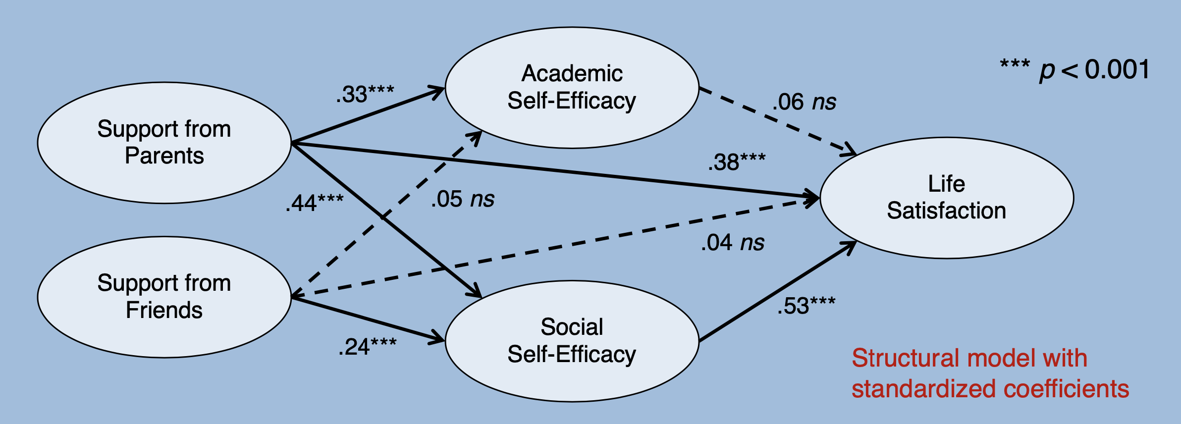
Summary of the indirect effects:
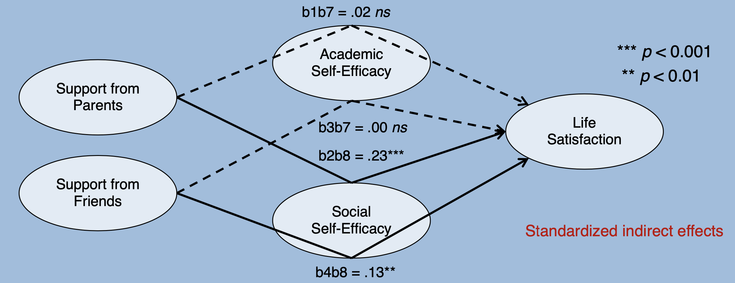
13.3 CFA and SEM with multiple groups
13.3.1 Measurement invariance analysis across multiple groups
Configural invariance
In a first step, the model is estimated with separate parameters for the two regional groups (“west”" and “east”), i.e. with twice as many model parameters. The overall model fit thus informs about a cross-group invariance with respect to the configural structure (e.g. a factor model with a certain number of factors and certain loadings etc.).
fit_configural <- sem(model_measurement,
                      data = data_sem,
                      estimator = "MLM",
                      group = "region")
summary(fit_configural, fit.measures = TRUE, standardized = TRUE)
## lavaan 0.6-9 ended normally after 64 iterations
##
## Estimator ML
## Optimization method NLMINB
## Number of model parameters 110
##
## Number of observations per group:
## west 141
## east 142
##
## Model Test User Model:
## Standard Robust
## Test Statistic 328.778 279.542
## Degrees of freedom 160 160
## P-value (Chi-square) 0.000 0.000
## Scaling correction factor 1.176
## Satorra-Bentler correction
## Test statistic for each group:
## west 170.704 145.141
## east 158.073 134.401
##
## Model Test Baseline Model:
##
## Test statistic 2786.197 1986.569
## Degrees of freedom 210 210
## P-value 0.000 0.000
## Scaling correction factor 1.403
##
## User Model versus Baseline Model:
##
## Comparative Fit Index (CFI) 0.934 0.933
## Tucker-Lewis Index (TLI) 0.914 0.912
##
## Robust Comparative Fit Index (CFI) 0.944
## Robust Tucker-Lewis Index (TLI) 0.926
##
## Loglikelihood and Information Criteria:
##
## Loglikelihood user model (H0) -4178.506 -4178.506
## Loglikelihood unrestricted model (H1) -4014.118 -4014.118
##
## Akaike (AIC) 8577.013 8577.013
## Bayesian (BIC) 8978.012 8978.012
## Sample-size adjusted Bayesian (BIC) 8629.201 8629.201
##
## Root Mean Square Error of Approximation:
##
## RMSEA 0.086 0.073
## 90 Percent confidence interval - lower 0.073 0.059
## 90 Percent confidence interval - upper 0.100 0.086
## P-value RMSEA <= 0.05 0.000 0.003
##
## Robust RMSEA 0.079
## 90 Percent confidence interval - lower 0.063
## 90 Percent confidence interval - upper 0.094
##
## Standardized Root Mean Square Residual:
##
## SRMR 0.061 0.061
##
## Parameter Estimates:
##
## Standard errors Robust.sem
## Information Expected
## Information saturated (h1) model Structured
##
##
## Group 1 [west]:
##
## Latent Variables:
## Estimate Std.Err z-value P(>|z|) Std.lv Std.all
## SUP_Parents =~
## sup_parents_p1 1.000 0.991 0.886
## sup_parents_p2 1.083 0.083 13.017 0.000 1.073 0.907
## sup_parents_p3 0.959 0.100 9.635 0.000 0.950 0.771
## SUP_Friends =~
## sup_friends_p1 1.000 1.169 0.914
## sup_friends_p2 0.794 0.082 9.660 0.000 0.929 0.844
## sup_friends_p3 0.913 0.111 8.189 0.000 1.067 0.834
## SE_Academic =~
## se_acad_p1 1.000 0.659 0.889
## se_acad_p2 0.783 0.063 12.398 0.000 0.516 0.788
## se_acad_p3 0.965 0.084 11.522 0.000 0.636 0.850
## SE_Social =~
## se_social_p1 1.000 0.615 0.845
## se_social_p2 1.027 0.095 10.795 0.000 0.632 0.854
## se_social_p3 0.884 0.109 8.107 0.000 0.544 0.707
## LS =~
## ls_p1 1.000 0.638 0.705
## ls_p2 0.777 0.119 6.503 0.000 0.496 0.682
## ls_p3 0.981 0.133 7.381 0.000 0.626 0.736
##
## Covariances:
## Estimate Std.Err z-value P(>|z|) Std.lv Std.all
## SUP_Parents ~~
## SUP_Friends 0.219 0.112 1.961 0.050 0.189 0.189
## SE_Academic 0.164 0.063 2.618 0.009 0.252 0.252
## SE_Social 0.209 0.061 3.448 0.001 0.344 0.344
## LS 0.340 0.061 5.609 0.000 0.537 0.537
## SUP_Friends ~~
## SE_Academic 0.012 0.071 0.171 0.865 0.016 0.016
## SE_Social 0.189 0.058 3.267 0.001 0.262 0.262
## LS 0.182 0.079 2.305 0.021 0.244 0.244
## SE_Academic ~~
## SE_Social 0.242 0.044 5.489 0.000 0.598 0.598
## LS 0.223 0.061 3.624 0.000 0.530 0.530
## SE_Social ~~
## LS 0.284 0.068 4.212 0.000 0.725 0.725
##
## Intercepts:
## Estimate Std.Err z-value P(>|z|) Std.lv Std.all
## .sup_parents_p1 5.947 0.094 63.141 0.000 5.947 5.317
## .sup_parents_p2 5.798 0.100 58.172 0.000 5.798 4.899
## .sup_parents_p3 5.574 0.104 53.734 0.000 5.574 4.525
## .sup_friends_p1 5.670 0.108 52.613 0.000 5.670 4.431
## .sup_friends_p2 5.901 0.093 63.697 0.000 5.901 5.364
## .sup_friends_p3 5.858 0.108 54.386 0.000 5.858 4.580
## .se_acad_p1 4.982 0.062 79.820 0.000 4.982 6.722
## .se_acad_p2 5.165 0.055 93.644 0.000 5.165 7.886
## .se_acad_p3 4.899 0.063 77.797 0.000 4.899 6.552
## .se_social_p1 5.216 0.061 85.032 0.000 5.216 7.161
## .se_social_p2 5.328 0.062 85.534 0.000 5.328 7.203
## .se_social_p3 5.273 0.065 81.305 0.000 5.273 6.847
## .ls_p1 5.163 0.076 67.748 0.000 5.163 5.705
## .ls_p2 5.709 0.061 93.294 0.000 5.709 7.857
## .ls_p3 4.973 0.072 69.489 0.000 4.973 5.852
## SUP_Parents 0.000 0.000 0.000
## SUP_Friends 0.000 0.000 0.000
## SE_Academic 0.000 0.000 0.000
## SE_Social 0.000 0.000 0.000
## LS 0.000 0.000 0.000
##
## Variances:
## Estimate Std.Err z-value P(>|z|) Std.lv Std.all
## .sup_parents_p1 0.269 0.065 4.121 0.000 0.269 0.215
## .sup_parents_p2 0.249 0.090 2.779 0.005 0.249 0.178
## .sup_parents_p3 0.615 0.130 4.744 0.000 0.615 0.405
## .sup_friends_p1 0.271 0.128 2.115 0.034 0.271 0.165
## .sup_friends_p2 0.347 0.102 3.401 0.001 0.347 0.287
## .sup_friends_p3 0.497 0.187 2.661 0.008 0.497 0.304
## .se_acad_p1 0.115 0.034 3.433 0.001 0.115 0.210
## .se_acad_p2 0.163 0.027 6.033 0.000 0.163 0.380
## .se_acad_p3 0.155 0.035 4.389 0.000 0.155 0.277
## .se_social_p1 0.152 0.026 5.911 0.000 0.152 0.287
## .se_social_p2 0.148 0.031 4.785 0.000 0.148 0.271
## .se_social_p3 0.297 0.040 7.467 0.000 0.297 0.501
## .ls_p1 0.412 0.066 6.241 0.000 0.412 0.503
## .ls_p2 0.283 0.100 2.837 0.005 0.283 0.535
## .ls_p3 0.330 0.049 6.683 0.000 0.330 0.458
## SUP_Parents 0.982 0.202 4.855 0.000 1.000 1.000
## SUP_Friends 1.367 0.253 5.402 0.000 1.000 1.000
## SE_Academic 0.434 0.069 6.264 0.000 1.000 1.000
## SE_Social 0.378 0.077 4.920 0.000 1.000 1.000
## LS 0.407 0.112 3.626 0.000 1.000 1.000
##
##
## Group 2 [east]:
##
## Latent Variables:
## Estimate Std.Err z-value P(>|z|) Std.lv Std.all
## SUP_Parents =~
## sup_parents_p1 1.000 0.894 0.875
## sup_parents_p2 0.943 0.078 12.081 0.000 0.843 0.863
## sup_parents_p3 0.984 0.076 12.951 0.000 0.880 0.857
## SUP_Friends =~
## sup_friends_p1 1.000 0.840 0.896
## sup_friends_p2 0.773 0.074 10.415 0.000 0.649 0.873
## sup_friends_p3 0.825 0.066 12.548 0.000 0.693 0.811
## SE_Academic =~
## se_acad_p1 1.000 0.700 0.873
## se_acad_p2 0.772 0.069 11.230 0.000 0.541 0.812
## se_acad_p3 0.807 0.082 9.812 0.000 0.565 0.777
## SE_Social =~
## se_social_p1 1.000 0.666 0.856
## se_social_p2 0.851 0.074 11.521 0.000 0.567 0.917
## se_social_p3 0.889 0.069 12.839 0.000 0.591 0.746
## LS =~
## ls_p1 1.000 0.726 0.764
## ls_p2 0.727 0.100 7.280 0.000 0.528 0.729
## ls_p3 0.843 0.109 7.708 0.000 0.611 0.725
##
## Covariances:
## Estimate Std.Err z-value P(>|z|) Std.lv Std.all
## SUP_Parents ~~
## SUP_Friends 0.025 0.070 0.358 0.720 0.033 0.033
## SE_Academic 0.250 0.063 3.978 0.000 0.399 0.399
## SE_Social 0.349 0.122 2.873 0.004 0.587 0.587
## LS 0.486 0.123 3.964 0.000 0.749 0.749
## SUP_Friends ~~
## SE_Academic 0.075 0.054 1.379 0.168 0.127 0.127
## SE_Social 0.179 0.048 3.726 0.000 0.321 0.321
## LS 0.142 0.057 2.490 0.013 0.233 0.233
## SE_Academic ~~
## SE_Social 0.268 0.054 4.981 0.000 0.576 0.576
## LS 0.228 0.059 3.870 0.000 0.449 0.449
## SE_Social ~~
## LS 0.361 0.086 4.186 0.000 0.747 0.747
##
## Intercepts:
## Estimate Std.Err z-value P(>|z|) Std.lv Std.all
## .sup_parents_p1 6.004 0.086 70.016 0.000 6.004 5.876
## .sup_parents_p2 6.056 0.082 73.867 0.000 6.056 6.199
## .sup_parents_p3 5.863 0.086 68.070 0.000 5.863 5.712
## .sup_friends_p1 5.901 0.079 75.067 0.000 5.901 6.299
## .sup_friends_p2 6.120 0.062 98.103 0.000 6.120 8.233
## .sup_friends_p3 6.123 0.072 85.429 0.000 6.123 7.169
## .se_acad_p1 5.327 0.067 79.100 0.000 5.327 6.638
## .se_acad_p2 5.527 0.056 98.863 0.000 5.527 8.296
## .se_acad_p3 5.521 0.061 90.458 0.000 5.521 7.591
## .se_social_p1 5.364 0.065 82.218 0.000 5.364 6.900
## .se_social_p2 5.626 0.052 108.519 0.000 5.626 9.107
## .se_social_p3 5.608 0.066 84.339 0.000 5.608 7.078
## .ls_p1 5.221 0.080 65.475 0.000 5.221 5.495
## .ls_p2 5.846 0.061 96.252 0.000 5.846 8.077
## .ls_p3 5.470 0.071 77.293 0.000 5.470 6.486
## SUP_Parents 0.000 0.000 0.000
## SUP_Friends 0.000 0.000 0.000
## SE_Academic 0.000 0.000 0.000
## SE_Social 0.000 0.000 0.000
## LS 0.000 0.000 0.000
##
## Variances:
## Estimate Std.Err z-value P(>|z|) Std.lv Std.all
## .sup_parents_p1 0.244 0.057 4.315 0.000 0.244 0.234
## .sup_parents_p2 0.244 0.054 4.486 0.000 0.244 0.255
## .sup_parents_p3 0.279 0.052 5.359 0.000 0.279 0.265
## .sup_friends_p1 0.173 0.058 2.972 0.003 0.173 0.197
## .sup_friends_p2 0.131 0.028 4.710 0.000 0.131 0.238
## .sup_friends_p3 0.249 0.058 4.310 0.000 0.249 0.342
## .se_acad_p1 0.154 0.040 3.841 0.000 0.154 0.238
## .se_acad_p2 0.151 0.030 4.979 0.000 0.151 0.341
## .se_acad_p3 0.210 0.039 5.342 0.000 0.210 0.397
## .se_social_p1 0.161 0.036 4.439 0.000 0.161 0.267
## .se_social_p2 0.061 0.016 3.828 0.000 0.061 0.159
## .se_social_p3 0.278 0.037 7.549 0.000 0.278 0.443
## .ls_p1 0.376 0.062 6.104 0.000 0.376 0.417
## .ls_p2 0.245 0.059 4.167 0.000 0.245 0.468
## .ls_p3 0.337 0.069 4.902 0.000 0.337 0.474
## SUP_Parents 0.800 0.211 3.784 0.000 1.000 1.000
## SUP_Friends 0.705 0.135 5.211 0.000 1.000 1.000
## SE_Academic 0.490 0.066 7.400 0.000 1.000 1.000
## SE_Social 0.443 0.102 4.354 0.000 1.000 1.000
## LS 0.526 0.106 4.962 0.000 1.000 1.000Metric (weak) measurement invariance
In the second step, the loading parameters of the measurement model are restricted to equality between the groups. The model fit and a model comparison with the previous model allow conclusions regarding the hypothesis of a “weak” (metric) measurement invariance across groups.
fit_metric <- sem(model_measurement,
                  data = data_sem,
                  estimator = "MLM",
                  group = "region",
                  group.equal = "loadings")
summary(fit_metric, fit.measures = TRUE, standardized = TRUE)
## lavaan 0.6-9 ended normally after 59 iterations
##
## Estimator ML
## Optimization method NLMINB
## Number of model parameters 110
## Number of equality constraints 10
##
## Number of observations per group:
## west 141
## east 142
##
## Model Test User Model:
## Standard Robust
## Test Statistic 338.264 286.015
## Degrees of freedom 170 170
## P-value (Chi-square) 0.000 0.000
## Scaling correction factor 1.183
## Satorra-Bentler correction
## Test statistic for each group:
## west 175.893 148.725
## east 162.370 137.290
##
## Model Test Baseline Model:
##
## Test statistic 2786.197 1986.569
## Degrees of freedom 210 210
## P-value 0.000 0.000
## Scaling correction factor 1.403
##
## User Model versus Baseline Model:
##
## Comparative Fit Index (CFI) 0.935 0.935
## Tucker-Lewis Index (TLI) 0.919 0.919
##
## Robust Comparative Fit Index (CFI) 0.945
## Robust Tucker-Lewis Index (TLI) 0.932
##
## Loglikelihood and Information Criteria:
##
## Loglikelihood user model (H0) -4183.249 -4183.249
## Loglikelihood unrestricted model (H1) -4014.118 -4014.118
##
## Akaike (AIC) 8566.499 8566.499
## Bayesian (BIC) 8931.043 8931.043
## Sample-size adjusted Bayesian (BIC) 8613.942 8613.942
##
## Root Mean Square Error of Approximation:
##
## RMSEA 0.084 0.069
## 90 Percent confidence interval - lower 0.071 0.056
## 90 Percent confidence interval - upper 0.097 0.082
## P-value RMSEA <= 0.05 0.000 0.009
##
## Robust RMSEA 0.076
## 90 Percent confidence interval - lower 0.060
## 90 Percent confidence interval - upper 0.091
##
## Standardized Root Mean Square Residual:
##
## SRMR 0.064 0.064
##
## Parameter Estimates:
##
## Standard errors Robust.sem
## Information Expected
## Information saturated (h1) model Structured
##
##
## Group 1 [west]:
##
## Latent Variables:
## Estimate Std.Err z-value P(>|z|) Std.lv Std.all
## SUP_Parents =~
## sp_pr_1 1.000 1.014 0.896
## sp_pr_2 (.p2.) 1.011 0.059 17.203 0.000 1.025 0.888
## sp_pr_3 (.p3.) 0.979 0.061 15.945 0.000 0.993 0.787
## SUP_Friends =~
## sp_fr_1 1.000 1.186 0.920
## sp_fr_2 (.p5.) 0.785 0.056 14.065 0.000 0.931 0.844
## sp_fr_3 (.p6.) 0.869 0.064 13.494 0.000 1.031 0.821
## SE_Academic =~
## s_cd_p1 1.000 0.675 0.900
## s_cd_p2 (.p8.) 0.781 0.047 16.619 0.000 0.527 0.794
## s_cd_p3 (.p9.) 0.891 0.058 15.320 0.000 0.601 0.827
## SE_Social =~
## s_scl_1 1.000 0.639 0.861
## s_scl_2 (.11.) 0.914 0.063 14.426 0.000 0.585 0.820
## s_scl_3 (.12.) 0.888 0.065 13.742 0.000 0.568 0.722
## LS =~
## ls_p1 1.000 0.666 0.725
## ls_p2 (.14.) 0.752 0.077 9.816 0.000 0.501 0.691
## ls_p3 (.15.) 0.897 0.082 10.921 0.000 0.597 0.712
##
## Covariances:
## Estimate Std.Err z-value P(>|z|) Std.lv Std.all
## SUP_Parents ~~
## SUP_Friends 0.226 0.113 1.999 0.046 0.188 0.188
## SE_Academic 0.174 0.065 2.672 0.008 0.254 0.254
## SE_Social 0.227 0.063 3.602 0.000 0.350 0.350
## LS 0.357 0.062 5.762 0.000 0.528 0.528
## SUP_Friends ~~
## SE_Academic 0.014 0.073 0.193 0.847 0.018 0.018
## SE_Social 0.194 0.061 3.179 0.001 0.255 0.255
## LS 0.189 0.085 2.234 0.026 0.240 0.240
## SE_Academic ~~
## SE_Social 0.263 0.043 6.165 0.000 0.611 0.611
## LS 0.234 0.060 3.886 0.000 0.521 0.521
## SE_Social ~~
## LS 0.312 0.066 4.729 0.000 0.732 0.732
##
## Intercepts:
## Estimate Std.Err z-value P(>|z|) Std.lv Std.all
## .sup_parents_p1 5.947 0.094 63.141 0.000 5.947 5.254
## .sup_parents_p2 5.798 0.100 58.172 0.000 5.798 5.022
## .sup_parents_p3 5.574 0.104 53.734 0.000 5.574 4.419
## .sup_friends_p1 5.670 0.108 52.613 0.000 5.670 4.398
## .sup_friends_p2 5.901 0.093 63.697 0.000 5.901 5.350
## .sup_friends_p3 5.858 0.108 54.386 0.000 5.858 4.665
## .se_acad_p1 4.982 0.062 79.820 0.000 4.982 6.647
## .se_acad_p2 5.165 0.055 93.644 0.000 5.165 7.785
## .se_acad_p3 4.899 0.063 77.797 0.000 4.899 6.742
## .se_social_p1 5.216 0.061 85.032 0.000 5.216 7.023
## .se_social_p2 5.328 0.062 85.534 0.000 5.328 7.474
## .se_social_p3 5.273 0.065 81.305 0.000 5.273 6.704
## .ls_p1 5.163 0.076 67.748 0.000 5.163 5.617
## .ls_p2 5.709 0.061 93.294 0.000 5.709 7.877
## .ls_p3 4.973 0.072 69.489 0.000 4.973 5.931
## SUP_Parents 0.000 0.000 0.000
## SUP_Friends 0.000 0.000 0.000
## SE_Academic 0.000 0.000 0.000
## SE_Social 0.000 0.000 0.000
## LS 0.000 0.000 0.000
##
## Variances:
## Estimate Std.Err z-value P(>|z|) Std.lv Std.all
## .sup_parents_p1 0.252 0.065 3.892 0.000 0.252 0.197
## .sup_parents_p2 0.281 0.085 3.321 0.001 0.281 0.211
## .sup_parents_p3 0.605 0.130 4.664 0.000 0.605 0.380
## .sup_friends_p1 0.256 0.121 2.109 0.035 0.256 0.154
## .sup_friends_p2 0.350 0.094 3.727 0.000 0.350 0.287
## .sup_friends_p3 0.514 0.173 2.969 0.003 0.514 0.326
## .se_acad_p1 0.107 0.033 3.278 0.001 0.107 0.190
## .se_acad_p2 0.163 0.027 6.024 0.000 0.163 0.370
## .se_acad_p3 0.167 0.032 5.207 0.000 0.167 0.315
## .se_social_p1 0.143 0.025 5.664 0.000 0.143 0.259
## .se_social_p2 0.166 0.029 5.789 0.000 0.166 0.327
## .se_social_p3 0.296 0.040 7.336 0.000 0.296 0.479
## .ls_p1 0.401 0.066 6.113 0.000 0.401 0.475
## .ls_p2 0.275 0.096 2.847 0.004 0.275 0.523
## .ls_p3 0.347 0.047 7.323 0.000 0.347 0.493
## SUP_Parents 1.029 0.189 5.436 0.000 1.000 1.000
## SUP_Friends 1.407 0.239 5.879 0.000 1.000 1.000
## SE_Academic 0.455 0.066 6.872 0.000 1.000 1.000
## SE_Social 0.409 0.074 5.491 0.000 1.000 1.000
## LS 0.444 0.101 4.405 0.000 1.000 1.000
##
##
## Group 2 [east]:
##
## Latent Variables:
## Estimate Std.Err z-value P(>|z|) Std.lv Std.all
## SUP_Parents =~
## sp_pr_1 1.000 0.873 0.867
## sp_pr_2 (.p2.) 1.011 0.059 17.203 0.000 0.883 0.878
## sp_pr_3 (.p3.) 0.979 0.061 15.945 0.000 0.855 0.847
## SUP_Friends =~
## sp_fr_1 1.000 0.825 0.889
## sp_fr_2 (.p5.) 0.785 0.056 14.065 0.000 0.647 0.873
## sp_fr_3 (.p6.) 0.869 0.064 13.494 0.000 0.717 0.824
## SE_Academic =~
## s_cd_p1 1.000 0.679 0.859
## s_cd_p2 (.p8.) 0.781 0.047 16.619 0.000 0.530 0.805
## s_cd_p3 (.p9.) 0.891 0.058 15.320 0.000 0.605 0.804
## SE_Social =~
## s_scl_1 1.000 0.639 0.839
## s_scl_2 (.11.) 0.914 0.063 14.426 0.000 0.584 0.930
## s_scl_3 (.12.) 0.888 0.065 13.742 0.000 0.567 0.730
## LS =~
## ls_p1 1.000 0.702 0.750
## ls_p2 (.14.) 0.752 0.077 9.816 0.000 0.528 0.728
## ls_p3 (.15.) 0.897 0.082 10.921 0.000 0.630 0.737
##
## Covariances:
## Estimate Std.Err z-value P(>|z|) Std.lv Std.all
## SUP_Parents ~~
## SUP_Friends 0.029 0.067 0.432 0.666 0.040 0.040
## SE_Academic 0.234 0.060 3.936 0.000 0.395 0.395
## SE_Social 0.326 0.107 3.029 0.002 0.584 0.584
## LS 0.462 0.116 3.983 0.000 0.754 0.754
## SUP_Friends ~~
## SE_Academic 0.071 0.052 1.364 0.173 0.127 0.127
## SE_Social 0.174 0.046 3.798 0.000 0.331 0.331
## LS 0.136 0.054 2.508 0.012 0.235 0.235
## SE_Academic ~~
## SE_Social 0.245 0.051 4.830 0.000 0.565 0.565
## LS 0.215 0.056 3.801 0.000 0.450 0.450
## SE_Social ~~
## LS 0.333 0.079 4.221 0.000 0.743 0.743
##
## Intercepts:
## Estimate Std.Err z-value P(>|z|) Std.lv Std.all
## .sup_parents_p1 6.004 0.086 70.016 0.000 6.004 5.962
## .sup_parents_p2 6.056 0.082 73.867 0.000 6.056 6.026
## .sup_parents_p3 5.863 0.086 68.070 0.000 5.863 5.809
## .sup_friends_p1 5.901 0.079 75.067 0.000 5.901 6.363
## .sup_friends_p2 6.120 0.062 98.103 0.000 6.120 8.251
## .sup_friends_p3 6.123 0.072 85.429 0.000 6.123 7.036
## .se_acad_p1 5.327 0.067 79.100 0.000 5.327 6.739
## .se_acad_p2 5.527 0.056 98.863 0.000 5.527 8.396
## .se_acad_p3 5.521 0.061 90.458 0.000 5.521 7.338
## .se_social_p1 5.364 0.065 82.218 0.000 5.364 7.048
## .se_social_p2 5.626 0.052 108.519 0.000 5.626 8.963
## .se_social_p3 5.608 0.066 84.339 0.000 5.608 7.218
## .ls_p1 5.221 0.080 65.475 0.000 5.221 5.572
## .ls_p2 5.846 0.061 96.252 0.000 5.846 8.058
## .ls_p3 5.470 0.071 77.293 0.000 5.470 6.405
## SUP_Parents 0.000 0.000 0.000
## SUP_Friends 0.000 0.000 0.000
## SE_Academic 0.000 0.000 0.000
## SE_Social 0.000 0.000 0.000
## LS 0.000 0.000 0.000
##
## Variances:
## Estimate Std.Err z-value P(>|z|) Std.lv Std.all
## .sup_parents_p1 0.252 0.052 4.853 0.000 0.252 0.248
## .sup_parents_p2 0.231 0.055 4.238 0.000 0.231 0.229
## .sup_parents_p3 0.288 0.052 5.570 0.000 0.288 0.282
## .sup_friends_p1 0.180 0.056 3.203 0.001 0.180 0.209
## .sup_friends_p2 0.131 0.025 5.206 0.000 0.131 0.238
## .sup_friends_p3 0.244 0.058 4.192 0.000 0.244 0.322
## .se_acad_p1 0.164 0.041 4.052 0.000 0.164 0.263
## .se_acad_p2 0.153 0.028 5.403 0.000 0.153 0.352
## .se_acad_p3 0.200 0.039 5.138 0.000 0.200 0.354
## .se_social_p1 0.171 0.035 4.909 0.000 0.171 0.296
## .se_social_p2 0.053 0.016 3.281 0.001 0.053 0.134
## .se_social_p3 0.282 0.037 7.666 0.000 0.282 0.468
## .ls_p1 0.385 0.063 6.078 0.000 0.385 0.438
## .ls_p2 0.247 0.058 4.250 0.000 0.247 0.470
## .ls_p3 0.333 0.069 4.807 0.000 0.333 0.456
## SUP_Parents 0.762 0.189 4.038 0.000 1.000 1.000
## SUP_Friends 0.680 0.123 5.542 0.000 1.000 1.000
## SE_Academic 0.461 0.064 7.240 0.000 1.000 1.000
## SE_Social 0.408 0.087 4.693 0.000 1.000 1.000
## LS 0.493 0.102 4.843 0.000 1.000 1.000anova(fit_configural, fit_metric)## Scaled Chi-Squared Difference Test (method = "satorra.bentler.2001")
##
## lavaan NOTE:
## The "Chisq" column contains standard test statistics, not the
## robust test that should be reported per model. A robust difference
## test is a function of two standard (not robust) statistics.
##
## Df AIC BIC Chisq Chisq diff Df diff Pr(>Chisq)
## fit_configural 160 8577.0 8978 328.78
## fit_metric 170 8566.5 8931 338.26 7.368 10 0.6903The comparison is not significant, thus metric measurement invariance can be assumed.
Scalar (strong) measurement invariance
In the next step, the intercepts of the manifest variables are additionally restricted to equality. Model fit and a model comparison with the previous model allow conclusions regarding the hypothesis of scalar (strong) measurement invariance. Scalar measurement invariance means that there is no differential item-functioning across groups.
However, this does not mean that a complete measurement invariance is guaranteed, because the procedure is not able to detect group-specific uniform response styles (all items of a construct affected by the same kind of bias).
fit_scalar <- sem(model_measurement,
                  data = data_sem,
                  estimator = "MLM",
                  group = "region",
                  group.equal = c("loadings", "intercepts"))
summary(fit_scalar, fit.measures = TRUE, standardized = TRUE)
## lavaan 0.6-9 ended normally after 137 iterations
##
## Estimator ML
## Optimization method NLMINB
## Number of model parameters 115
## Number of equality constraints 25
##
## Number of observations per group:
## west 141
## east 142
##
## Model Test User Model:
## Standard Robust
## Test Statistic 397.337 347.114
## Degrees of freedom 180 180
## P-value (Chi-square) 0.000 0.000
## Scaling correction factor 1.145
## Satorra-Bentler correction
## Test statistic for each group:
## west 200.588 175.234
## east 196.749 171.880
##
## Model Test Baseline Model:
##
## Test statistic 2786.197 1986.569
## Degrees of freedom 210 210
## P-value 0.000 0.000
## Scaling correction factor 1.403
##
## User Model versus Baseline Model:
##
## Comparative Fit Index (CFI) 0.916 0.906
## Tucker-Lewis Index (TLI) 0.902 0.890
##
## Robust Comparative Fit Index (CFI) 0.923
## Robust Tucker-Lewis Index (TLI) 0.910
##
## Loglikelihood and Information Criteria:
##
## Loglikelihood user model (H0) -4212.786 -4212.786
## Loglikelihood unrestricted model (H1) -4014.118 -4014.118
##
## Akaike (AIC) 8605.572 8605.572
## Bayesian (BIC) 8933.662 8933.662
## Sample-size adjusted Bayesian (BIC) 8648.271 8648.271
##
## Root Mean Square Error of Approximation:
##
## RMSEA 0.092 0.081
## 90 Percent confidence interval - lower 0.080 0.069
## 90 Percent confidence interval - upper 0.105 0.093
## P-value RMSEA <= 0.05 0.000 0.000
##
## Robust RMSEA 0.087
## 90 Percent confidence interval - lower 0.073
## 90 Percent confidence interval - upper 0.100
##
## Standardized Root Mean Square Residual:
##
## SRMR 0.070 0.070
##
## Parameter Estimates:
##
## Standard errors Robust.sem
## Information Expected
## Information saturated (h1) model Structured
##
##
## Group 1 [west]:
##
## Latent Variables:
## Estimate Std.Err z-value P(>|z|) Std.lv Std.all
## SUP_Parents =~
## sp_pr_1 1.000 1.003 0.888
## sp_pr_2 (.p2.) 1.030 0.059 17.363 0.000 1.033 0.891
## sp_pr_3 (.p3.) 0.999 0.064 15.712 0.000 1.002 0.790
## SUP_Friends =~
## sp_fr_1 1.000 1.183 0.919
## sp_fr_2 (.p5.) 0.789 0.055 14.253 0.000 0.933 0.845
## sp_fr_3 (.p6.) 0.875 0.065 13.511 0.000 1.035 0.822
## SE_Academic =~
## s_cd_p1 1.000 0.643 0.876
## s_cd_p2 (.p8.) 0.823 0.045 18.446 0.000 0.529 0.799
## s_cd_p3 (.p9.) 0.995 0.059 16.934 0.000 0.640 0.847
## SE_Social =~
## s_scl_1 1.000 0.622 0.845
## s_scl_2 (.11.) 0.958 0.065 14.624 0.000 0.596 0.828
## s_scl_3 (.12.) 0.936 0.068 13.818 0.000 0.583 0.733
## LS =~
## ls_p1 1.000 0.634 0.695
## ls_p2 (.14.) 0.773 0.073 10.533 0.000 0.490 0.678
## ls_p3 (.15.) 0.985 0.085 11.648 0.000 0.624 0.723
##
## Covariances:
## Estimate Std.Err z-value P(>|z|) Std.lv Std.all
## SUP_Parents ~~
## SUP_Friends 0.221 0.112 1.975 0.048 0.187 0.187
## SE_Academic 0.166 0.062 2.671 0.008 0.258 0.258
## SE_Social 0.218 0.061 3.574 0.000 0.349 0.349
## LS 0.345 0.060 5.785 0.000 0.543 0.543
## SUP_Friends ~~
## SE_Academic 0.011 0.070 0.154 0.878 0.014 0.014
## SE_Social 0.193 0.059 3.281 0.001 0.262 0.262
## LS 0.184 0.081 2.274 0.023 0.246 0.246
## SE_Academic ~~
## SE_Social 0.243 0.041 5.988 0.000 0.607 0.607
## LS 0.216 0.055 3.912 0.000 0.531 0.531
## SE_Social ~~
## LS 0.291 0.063 4.651 0.000 0.737 0.737
##
## Intercepts:
## Estimate Std.Err z-value P(>|z|) Std.lv Std.all
## .sp_pr_1 (.46.) 5.881 0.092 63.988 0.000 5.881 5.209
## .sp_pr_2 (.47.) 5.834 0.096 61.080 0.000 5.834 5.035
## .sp_pr_3 (.48.) 5.643 0.095 59.667 0.000 5.643 4.449
## .sp_fr_1 (.49.) 5.653 0.106 53.463 0.000 5.653 4.390
## .sp_fr_2 (.50.) 5.911 0.087 67.816 0.000 5.911 5.353
## .sp_fr_3 (.51.) 5.884 0.098 59.785 0.000 5.884 4.676
## .s_cd_p1 (.52.) 4.934 0.061 80.488 0.000 4.934 6.720
## .s_cd_p2 (.53.) 5.155 0.053 97.691 0.000 5.155 7.782
## .s_cd_p3 (.54.) 4.969 0.061 81.104 0.000 4.969 6.581
## .s_scl_1 (.55.) 5.162 0.059 86.932 0.000 5.162 7.006
## .s_scl_2 (.56.) 5.362 0.059 91.279 0.000 5.362 7.453
## .s_scl_3 (.57.) 5.317 0.060 89.151 0.000 5.317 6.687
## .ls_p1 (.58.) 5.059 0.070 72.023 0.000 5.059 5.550
## .ls_p2 (.59.) 5.675 0.056 101.151 0.000 5.675 7.854
## .ls_p3 (.60.) 5.095 0.067 76.322 0.000 5.095 5.902
## SUP_Prn 0.000 0.000 0.000
## SUP_Frn 0.000 0.000 0.000
## SE_Acdm 0.000 0.000 0.000
## SE_Socl 0.000 0.000 0.000
## LS 0.000 0.000 0.000
##
## Variances:
## Estimate Std.Err z-value P(>|z|) Std.lv Std.all
## .sup_parents_p1 0.269 0.064 4.178 0.000 0.269 0.211
## .sup_parents_p2 0.276 0.084 3.288 0.001 0.276 0.206
## .sup_parents_p3 0.605 0.129 4.681 0.000 0.605 0.376
## .sup_friends_p1 0.259 0.119 2.179 0.029 0.259 0.156
## .sup_friends_p2 0.349 0.094 3.702 0.000 0.349 0.286
## .sup_friends_p3 0.512 0.172 2.972 0.003 0.512 0.324
## .se_acad_p1 0.126 0.030 4.136 0.000 0.126 0.233
## .se_acad_p2 0.159 0.027 5.954 0.000 0.159 0.362
## .se_acad_p3 0.161 0.033 4.850 0.000 0.161 0.282
## .se_social_p1 0.156 0.025 6.315 0.000 0.156 0.287
## .se_social_p2 0.162 0.029 5.660 0.000 0.162 0.314
## .se_social_p3 0.293 0.040 7.236 0.000 0.293 0.463
## .ls_p1 0.429 0.064 6.703 0.000 0.429 0.517
## .ls_p2 0.282 0.096 2.935 0.003 0.282 0.540
## .ls_p3 0.356 0.047 7.555 0.000 0.356 0.477
## SUP_Parents 1.006 0.187 5.384 0.000 1.000 1.000
## SUP_Friends 1.399 0.237 5.900 0.000 1.000 1.000
## SE_Academic 0.414 0.061 6.730 0.000 1.000 1.000
## SE_Social 0.387 0.071 5.419 0.000 1.000 1.000
## LS 0.402 0.094 4.280 0.000 1.000 1.000
##
##
## Group 2 [east]:
##
## Latent Variables:
## Estimate Std.Err z-value P(>|z|) Std.lv Std.all
## SUP_Parents =~
## sp_pr_1 1.000 0.861 0.859
## sp_pr_2 (.p2.) 1.030 0.059 17.363 0.000 0.886 0.879
## sp_pr_3 (.p3.) 0.999 0.064 15.712 0.000 0.860 0.849
## SUP_Friends =~
## sp_fr_1 1.000 0.822 0.888
## sp_fr_2 (.p5.) 0.789 0.055 14.253 0.000 0.648 0.873
## sp_fr_3 (.p6.) 0.875 0.065 13.511 0.000 0.719 0.825
## SE_Academic =~
## s_cd_p1 1.000 0.640 0.826
## s_cd_p2 (.p8.) 0.823 0.045 18.446 0.000 0.527 0.805
## s_cd_p3 (.p9.) 0.995 0.059 16.934 0.000 0.637 0.814
## SE_Social =~
## s_scl_1 1.000 0.615 0.820
## s_scl_2 (.11.) 0.958 0.065 14.624 0.000 0.589 0.936
## s_scl_3 (.12.) 0.936 0.068 13.818 0.000 0.576 0.734
## LS =~
## ls_p1 1.000 0.667 0.719
## ls_p2 (.14.) 0.773 0.073 10.533 0.000 0.516 0.716
## ls_p3 (.15.) 0.985 0.085 11.648 0.000 0.657 0.745
##
## Covariances:
## Estimate Std.Err z-value P(>|z|) Std.lv Std.all
## SUP_Parents ~~
## SUP_Friends 0.028 0.066 0.424 0.672 0.039 0.039
## SE_Academic 0.218 0.057 3.853 0.000 0.396 0.396
## SE_Social 0.307 0.102 3.021 0.003 0.579 0.579
## LS 0.439 0.112 3.923 0.000 0.765 0.765
## SUP_Friends ~~
## SE_Academic 0.068 0.049 1.373 0.170 0.129 0.129
## SE_Social 0.171 0.044 3.878 0.000 0.338 0.338
## LS 0.129 0.052 2.506 0.012 0.236 0.236
## SE_Academic ~~
## SE_Social 0.221 0.048 4.637 0.000 0.560 0.560
## LS 0.195 0.052 3.739 0.000 0.457 0.457
## SE_Social ~~
## LS 0.306 0.074 4.147 0.000 0.746 0.746
##
## Intercepts:
## Estimate Std.Err z-value P(>|z|) Std.lv Std.all
## .sp_pr_1 (.46.) 5.881 0.092 63.988 0.000 5.881 5.866
## .sp_pr_2 (.47.) 5.834 0.096 61.080 0.000 5.834 5.787
## .sp_pr_3 (.48.) 5.643 0.095 59.667 0.000 5.643 5.572
## .sp_fr_1 (.49.) 5.653 0.106 53.463 0.000 5.653 6.105
## .sp_fr_2 (.50.) 5.911 0.087 67.816 0.000 5.911 7.964
## .sp_fr_3 (.51.) 5.884 0.098 59.785 0.000 5.884 6.748
## .s_cd_p1 (.52.) 4.934 0.061 80.488 0.000 4.934 6.366
## .s_cd_p2 (.53.) 5.155 0.053 97.691 0.000 5.155 7.885
## .s_cd_p3 (.54.) 4.969 0.061 81.104 0.000 4.969 6.351
## .s_scl_1 (.55.) 5.162 0.059 86.932 0.000 5.162 6.877
## .s_scl_2 (.56.) 5.362 0.059 91.279 0.000 5.362 8.520
## .s_scl_3 (.57.) 5.317 0.060 89.151 0.000 5.317 6.780
## .ls_p1 (.58.) 5.059 0.070 72.023 0.000 5.059 5.457
## .ls_p2 (.59.) 5.675 0.056 101.151 0.000 5.675 7.879
## .ls_p3 (.60.) 5.095 0.067 76.322 0.000 5.095 5.777
## SUP_Prn 0.188 0.117 1.605 0.108 0.218 0.218
## SUP_Frn 0.260 0.127 2.048 0.041 0.317 0.317
## SE_Acdm 0.465 0.084 5.521 0.000 0.726 0.726
## SE_Socl 0.265 0.079 3.342 0.001 0.430 0.430
## LS 0.261 0.090 2.886 0.004 0.392 0.392
##
## Variances:
## Estimate Std.Err z-value P(>|z|) Std.lv Std.all
## .sup_parents_p1 0.264 0.051 5.174 0.000 0.264 0.263
## .sup_parents_p2 0.231 0.055 4.207 0.000 0.231 0.227
## .sup_parents_p3 0.286 0.052 5.485 0.000 0.286 0.279
## .sup_friends_p1 0.182 0.056 3.221 0.001 0.182 0.212
## .sup_friends_p2 0.131 0.025 5.184 0.000 0.131 0.237
## .sup_friends_p3 0.243 0.058 4.164 0.000 0.243 0.320
## .se_acad_p1 0.191 0.042 4.535 0.000 0.191 0.318
## .se_acad_p2 0.150 0.028 5.287 0.000 0.150 0.351
## .se_acad_p3 0.207 0.041 5.068 0.000 0.207 0.338
## .se_social_p1 0.185 0.035 5.284 0.000 0.185 0.328
## .se_social_p2 0.049 0.016 2.997 0.003 0.049 0.124
## .se_social_p3 0.283 0.037 7.721 0.000 0.283 0.461
## .ls_p1 0.415 0.064 6.478 0.000 0.415 0.483
## .ls_p2 0.253 0.058 4.349 0.000 0.253 0.487
## .ls_p3 0.347 0.071 4.876 0.000 0.347 0.446
## SUP_Parents 0.741 0.185 4.010 0.000 1.000 1.000
## SUP_Friends 0.676 0.122 5.555 0.000 1.000 1.000
## SE_Academic 0.410 0.060 6.886 0.000 1.000 1.000
## SE_Social 0.378 0.081 4.662 0.000 1.000 1.000
## LS 0.445 0.096 4.615 0.000 1.000 1.000anova(fit_metric, fit_scalar)## Scaled Chi-Squared Difference Test (method = "satorra.bentler.2001")
##
## lavaan NOTE:
## The "Chisq" column contains standard test statistics, not the
## robust test that should be reported per model. A robust difference
## test is a function of two standard (not robust) statistics.
##
## Df AIC BIC Chisq Chisq diff Df diff Pr(>Chisq)
## fit_metric 170 8566.5 8931.0 338.26
## fit_scalar 180 8605.6 8933.7 397.34 118.43 10 < 2.2e-16 ***
## ---
## Signif. codes: 0 '***' 0.001 '**' 0.01 '*' 0.05 '.' 0.1 ' ' 1This time the comparison is highly significant. The assumption of identical intercepts and thus “strong” (scalar) measurement invariance must therefore be rejected. Another criterion frequently cited in the literature is that the more restrictive model (despite the significant chi-square value) should only have a CFI/TLI that is less 0.01 lower than the CFI/TLI of the less restrictive model.
m <- fitMeasures(fit_metric)[names = c("cfi.robust", "tli.robust")]
s <- fitMeasures(fit_scalar)[names = c("cfi.robust", "tli.robust")]
round(m - s, 3)
## cfi.robust tli.robust
## 0.022 0.022Here we are above this cut-off value. Thus, strong measurement invariance is not supported.
13.3.2 Multi-group analyses for the structural model (moderation analyses)
In addition to measurement invariance, multi-group analysis can be used to check the invariance of structural paths. This allows to check moderation hypotheses (group variables as moderators) for single or multiple structural paths.
First, however, a procedure is presented that checks the entire structural model (i.e. all structural path coefficients) for equivalence (in addition to the weak measurement invariance).
Overall moderation test / equivalence of the structural model across groups
fit_allequal <- sem(model,
                    data = data_sem,
                    estimator = "MLM",
                    group = "region",
                    group.equal = c("loadings", "regressions"))
This model is often compared to the weak (and not the strong) measurement invariance model because for CFAs/SEMs where the mean structure is not of interest the metric measurement invariance (equivalence of factor loadings) is sufficient.
We first have to estimate the full model with metric equivalence restrictions (which we have done so far only for the measurement model):
fit_structure_metric <- sem(model,
                    data = data_sem,
                    estimator = "MLM",
                    group = "region",
                    group.equal = c("loadings"))

summary(fit_structure_metric, fit.measures = TRUE, standardized = TRUE)
## lavaan 0.6-9 ended normally after 50 iterations
##
## Estimator ML
## Optimization method NLMINB
## Number of model parameters 110
## Number of equality constraints 10
##
## Number of observations per group:
## west 141
## east 142
##
## Model Test User Model:
## Standard Robust
## Test Statistic 338.264 286.015
## Degrees of freedom 170 170
## P-value (Chi-square) 0.000 0.000
## Scaling correction factor 1.183
## Satorra-Bentler correction
## Test statistic for each group:
## west 175.893 148.724
## east 162.370 137.290
##
## Model Test Baseline Model:
##
## Test statistic 2786.197 1986.569
## Degrees of freedom 210 210
## P-value 0.000 0.000
## Scaling correction factor 1.403
##
## User Model versus Baseline Model:
##
## Comparative Fit Index (CFI) 0.935 0.935
## Tucker-Lewis Index (TLI) 0.919 0.919
##
## Robust Comparative Fit Index (CFI) 0.945
## Robust Tucker-Lewis Index (TLI) 0.932
##
## Loglikelihood and Information Criteria:
##
## Loglikelihood user model (H0) -4183.249 -4183.249
## Loglikelihood unrestricted model (H1) -4014.118 -4014.118
##
## Akaike (AIC) 8566.499 8566.499
## Bayesian (BIC) 8931.043 8931.043
## Sample-size adjusted Bayesian (BIC) 8613.942 8613.942
##
## Root Mean Square Error of Approximation:
##
## RMSEA 0.084 0.069
## 90 Percent confidence interval - lower 0.071 0.056
## 90 Percent confidence interval - upper 0.097 0.082
## P-value RMSEA <= 0.05 0.000 0.009
##
## Robust RMSEA 0.076
## 90 Percent confidence interval - lower 0.060
## 90 Percent confidence interval - upper 0.091
##
## Standardized Root Mean Square Residual:
##
## SRMR 0.064 0.064
##
## Parameter Estimates:
##
## Standard errors Robust.sem
## Information Expected
## Information saturated (h1) model Structured
##
##
## Group 1 [west]:
##
## Latent Variables:
## Estimate Std.Err z-value P(>|z|) Std.lv Std.all
## SUP_Parents =~
## sp_pr_1 1.000 1.014 0.896
## sp_pr_2 (.p2.) 1.011 0.059 17.203 0.000 1.025 0.888
## sp_pr_3 (.p3.) 0.979 0.061 15.945 0.000 0.993 0.787
## SUP_Friends =~
## sp_fr_1 1.000 1.186 0.920
## sp_fr_2 (.p5.) 0.785 0.056 14.065 0.000 0.931 0.844
## sp_fr_3 (.p6.) 0.869 0.064 13.494 0.000 1.031 0.821
## SE_Academic =~
## s_cd_p1 1.000 0.675 0.900
## s_cd_p2 (.p8.) 0.781 0.047 16.619 0.000 0.527 0.794
## s_cd_p3 (.p9.) 0.891 0.058 15.320 0.000 0.601 0.827
## SE_Social =~
## s_scl_1 1.000 0.639 0.861
## s_scl_2 (.11.) 0.914 0.063 14.426 0.000 0.585 0.820
## s_scl_3 (.12.) 0.888 0.065 13.742 0.000 0.568 0.722
## LS =~
## ls_p1 1.000 0.666 0.725
## ls_p2 (.14.) 0.752 0.077 9.816 0.000 0.501 0.691
## ls_p3 (.15.) 0.897 0.082 10.921 0.000 0.597 0.712
##
## Regressions:
## Estimate Std.Err z-value P(>|z|) Std.lv Std.all
## SE_Academic ~
## SUP_Parents 0.173 0.074 2.347 0.019 0.260 0.260
## SUP_Friends -0.018 0.054 -0.328 0.743 -0.031 -0.031
## SE_Social ~
## SUP_Parents 0.197 0.071 2.772 0.006 0.313 0.313
## SUP_Friends 0.106 0.045 2.331 0.020 0.197 0.197
## LS ~
## SE_Academic 0.107 0.111 0.963 0.336 0.108 0.108
## SE_Social 0.574 0.125 4.596 0.000 0.551 0.551
## SUP_Parents 0.197 0.052 3.804 0.000 0.300 0.300
## SUP_Friends 0.023 0.049 0.470 0.639 0.041 0.041
##
## Covariances:
## Estimate Std.Err z-value P(>|z|) Std.lv Std.all
## .SE_Academic ~~
## .SE_Social 0.228 0.038 5.952 0.000 0.596 0.596
## SUP_Parents ~~
## SUP_Friends 0.226 0.113 1.999 0.046 0.188 0.188
##
## Intercepts:
## Estimate Std.Err z-value P(>|z|) Std.lv Std.all
## .sup_parents_p1 5.947 0.094 63.141 0.000 5.947 5.254
## .sup_parents_p2 5.798 0.100 58.172 0.000 5.798 5.022
## .sup_parents_p3 5.574 0.104 53.734 0.000 5.574 4.419
## .sup_friends_p1 5.670 0.108 52.613 0.000 5.670 4.398
## .sup_friends_p2 5.901 0.093 63.697 0.000 5.901 5.350
## .sup_friends_p3 5.858 0.108 54.386 0.000 5.858 4.665
## .se_acad_p1 4.982 0.062 79.820 0.000 4.982 6.647
## .se_acad_p2 5.165 0.055 93.644 0.000 5.165 7.785
## .se_acad_p3 4.899 0.063 77.797 0.000 4.899 6.742
## .se_social_p1 5.216 0.061 85.032 0.000 5.216 7.023
## .se_social_p2 5.328 0.062 85.534 0.000 5.328 7.474
## .se_social_p3 5.273 0.065 81.305 0.000 5.273 6.704
## .ls_p1 5.163 0.076 67.748 0.000 5.163 5.617
## .ls_p2 5.709 0.061 93.294 0.000 5.709 7.877
## .ls_p3 4.973 0.072 69.489 0.000 4.973 5.931
## SUP_Parents 0.000 0.000 0.000
## SUP_Friends 0.000 0.000 0.000
## .SE_Academic 0.000 0.000 0.000
## .SE_Social 0.000 0.000 0.000
## .LS 0.000 0.000 0.000
##
## Variances:
## Estimate Std.Err z-value P(>|z|) Std.lv Std.all
## .sup_parents_p1 0.252 0.065 3.892 0.000 0.252 0.197
## .sup_parents_p2 0.281 0.085 3.321 0.001 0.281 0.211
## .sup_parents_p3 0.605 0.130 4.664 0.000 0.605 0.380
## .sup_friends_p1 0.256 0.121 2.109 0.035 0.256 0.154
## .sup_friends_p2 0.350 0.094 3.727 0.000 0.350 0.287
## .sup_friends_p3 0.514 0.173 2.969 0.003 0.514 0.326
## .se_acad_p1 0.107 0.033 3.278 0.001 0.107 0.190
## .se_acad_p2 0.163 0.027 6.024 0.000 0.163 0.370
## .se_acad_p3 0.167 0.032 5.207 0.000 0.167 0.315
## .se_social_p1 0.143 0.025 5.664 0.000 0.143 0.259
## .se_social_p2 0.166 0.029 5.789 0.000 0.166 0.327
## .se_social_p3 0.296 0.040 7.336 0.000 0.296 0.479
## .ls_p1 0.401 0.066 6.113 0.000 0.401 0.475
## .ls_p2 0.275 0.096 2.847 0.004 0.275 0.523
## .ls_p3 0.347 0.047 7.323 0.000 0.347 0.493
## SUP_Parents 1.029 0.189 5.436 0.000 1.000 1.000
## SUP_Friends 1.407 0.239 5.879 0.000 1.000 1.000
## .SE_Academic 0.425 0.060 7.124 0.000 0.935 0.935
## .SE_Social 0.344 0.060 5.729 0.000 0.840 0.840
## .LS 0.165 0.047 3.523 0.000 0.372 0.372
##
##
## Group 2 [east]:
##
## Latent Variables:
## Estimate Std.Err z-value P(>|z|) Std.lv Std.all
## SUP_Parents =~
## sp_pr_1 1.000 0.873 0.867
## sp_pr_2 (.p2.) 1.011 0.059 17.203 0.000 0.883 0.878
## sp_pr_3 (.p3.) 0.979 0.061 15.945 0.000 0.855 0.847
## SUP_Friends =~
## sp_fr_1 1.000 0.825 0.889
## sp_fr_2 (.p5.) 0.785 0.056 14.065 0.000 0.647 0.873
## sp_fr_3 (.p6.) 0.869 0.064 13.494 0.000 0.717 0.824
## SE_Academic =~
## s_cd_p1 1.000 0.679 0.859
## s_cd_p2 (.p8.) 0.781 0.047 16.619 0.000 0.530 0.805
## s_cd_p3 (.p9.) 0.891 0.058 15.320 0.000 0.605 0.804
## SE_Social =~
## s_scl_1 1.000 0.639 0.839
## s_scl_2 (.11.) 0.914 0.063 14.426 0.000 0.584 0.930
## s_scl_3 (.12.) 0.888 0.065 13.742 0.000 0.567 0.730
## LS =~
## ls_p1 1.000 0.702 0.750
## ls_p2 (.14.) 0.752 0.077 9.816 0.000 0.528 0.728
## ls_p3 (.15.) 0.897 0.082 10.921 0.000 0.630 0.737
##
## Regressions:
## Estimate Std.Err z-value P(>|z|) Std.lv Std.all
## SE_Academic ~
## SUP_Parents 0.304 0.068 4.468 0.000 0.391 0.391
## SUP_Friends 0.091 0.071 1.279 0.201 0.111 0.111
## SE_Social ~
## SUP_Parents 0.418 0.081 5.166 0.000 0.572 0.572
## SUP_Friends 0.238 0.052 4.621 0.000 0.308 0.308
## LS ~
## SE_Academic 0.003 0.112 0.025 0.980 0.003 0.003
## SE_Social 0.466 0.116 4.006 0.000 0.424 0.424
## SUP_Parents 0.404 0.083 4.847 0.000 0.502 0.502
## SUP_Friends 0.063 0.052 1.226 0.220 0.074 0.074
##
## Covariances:
## Estimate Std.Err z-value P(>|z|) Std.lv Std.all
## .SE_Academic ~~
## .SE_Social 0.130 0.031 4.240 0.000 0.438 0.438
## SUP_Parents ~~
## SUP_Friends 0.029 0.067 0.432 0.666 0.040 0.040
##
## Intercepts:
## Estimate Std.Err z-value P(>|z|) Std.lv Std.all
## .sup_parents_p1 6.004 0.086 70.016 0.000 6.004 5.962
## .sup_parents_p2 6.056 0.082 73.867 0.000 6.056 6.026
## .sup_parents_p3 5.863 0.086 68.070 0.000 5.863 5.809
## .sup_friends_p1 5.901 0.079 75.067 0.000 5.901 6.363
## .sup_friends_p2 6.120 0.062 98.103 0.000 6.120 8.251
## .sup_friends_p3 6.123 0.072 85.429 0.000 6.123 7.036
## .se_acad_p1 5.327 0.067 79.100 0.000 5.327 6.739
## .se_acad_p2 5.527 0.056 98.863 0.000 5.527 8.396
## .se_acad_p3 5.521 0.061 90.458 0.000 5.521 7.338
## .se_social_p1 5.364 0.065 82.218 0.000 5.364 7.048
## .se_social_p2 5.626 0.052 108.519 0.000 5.626 8.963
## .se_social_p3 5.608 0.066 84.339 0.000 5.608 7.218
## .ls_p1 5.221 0.080 65.475 0.000 5.221 5.572
## .ls_p2 5.846 0.061 96.252 0.000 5.846 8.058
## .ls_p3 5.470 0.071 77.293 0.000 5.470 6.405
## SUP_Parents 0.000 0.000 0.000
## SUP_Friends 0.000 0.000 0.000
## .SE_Academic 0.000 0.000 0.000
## .SE_Social 0.000 0.000 0.000
## .LS 0.000 0.000 0.000
##
## Variances:
## Estimate Std.Err z-value P(>|z|) Std.lv Std.all
## .sup_parents_p1 0.252 0.052 4.853 0.000 0.252 0.248
## .sup_parents_p2 0.231 0.055 4.238 0.000 0.231 0.229
## .sup_parents_p3 0.288 0.052 5.570 0.000 0.288 0.282
## .sup_friends_p1 0.180 0.056 3.203 0.001 0.180 0.209
## .sup_friends_p2 0.131 0.025 5.206 0.000 0.131 0.238
## .sup_friends_p3 0.244 0.058 4.192 0.000 0.244 0.322
## .se_acad_p1 0.164 0.041 4.052 0.000 0.164 0.263
## .se_acad_p2 0.153 0.028 5.403 0.000 0.153 0.352
## .se_acad_p3 0.200 0.039 5.138 0.000 0.200 0.354
## .se_social_p1 0.171 0.035 4.909 0.000 0.171 0.296
## .se_social_p2 0.053 0.016 3.281 0.001 0.053 0.134
## .se_social_p3 0.282 0.037 7.666 0.000 0.282 0.468
## .ls_p1 0.385 0.063 6.078 0.000 0.385 0.438
## .ls_p2 0.247 0.058 4.250 0.000 0.247 0.470
## .ls_p3 0.333 0.069 4.807 0.000 0.333 0.456
## SUP_Parents 0.762 0.189 4.038 0.000 1.000 1.000
## SUP_Friends 0.680 0.123 5.542 0.000 1.000 1.000
## .SE_Academic 0.383 0.060 6.361 0.000 0.831 0.831
## .SE_Social 0.230 0.043 5.340 0.000 0.565 0.565
## .LS 0.142 0.043 3.326 0.001 0.288 0.288Now we can compare with the equal structural paths model:
anova(fit_structure_metric, fit_allequal)## Scaled Chi-Squared Difference Test (method = "satorra.bentler.2001")
##
## lavaan NOTE:
## The "Chisq" column contains standard test statistics, not the
## robust test that should be reported per model. A robust difference
## test is a function of two standard (not robust) statistics.
##
## Df AIC BIC Chisq Chisq diff Df diff Pr(>Chisq)
## fit_structure_metric 170 8566.5 8931.0 338.26
## fit_allequal 178 8568.0 8903.4 355.74 15.768 8 0.04582 *
## ---
## Signif. codes: 0 '***' 0.001 '**' 0.01 '*' 0.05 '.' 0.1 ' ' 1The \(H_0\) that all parameters related to the structural model are equal across East and West German adolescents has to be rejected. In the following, we try to pinpoint the moderation effect with regard to the structural path coefficients.
Moderated mediation analysis
We can conduct a moderated mediation analysis by using a group variable (factor) as a moderator variable for the paths in the structural model.
In order to test the differences of individual paths between the groups (moderation), we need an alternative method for equality constraints based on explicit naming of the individual parameters.
We will show this first for all 8 regression paths individually, and then for the 4 combined paths representing the specific indirect effects in the model.
Moderation tests for the 8 individual paths
1) Support from Parents \(\rightarrow\) Academic Self-Efficacy
model_b1 <- '
# Measurement model
SUP_Parents =~ sup_parents_p1 + sup_parents_p2 + sup_parents_p3
SUP_Friends =~ sup_friends_p1 + sup_friends_p2 + sup_friends_p3
SE_Academic =~ se_acad_p1 + se_acad_p2 + se_acad_p3
SE_Social =~ se_social_p1 + se_social_p2 + se_social_p3
LS  =~ ls_p1 + ls_p2 + ls_p3

# Structural model
# Regressions
SE_Academic ~ c(b1, b1)*SUP_Parents + SUP_Friends
SE_Social ~ SUP_Parents + SUP_Friends
LS ~ SUP_Parents + SUP_Friends + SE_Academic + SE_Social

# Residual covariances
SE_Academic ~~ SE_Social
'

fit_b1 <- sem(model_b1,
              data = data_sem,
              estimator = "MLM",
              group = "region",
              group.equal = "loadings")
anova(fit_b1, fit_structure_metric)
## Scaled Chi-Squared Difference Test (method = "satorra.bentler.2001")
##
## lavaan NOTE:
## The "Chisq" column contains standard test statistics, not the
## robust test that should be reported per model. A robust difference
## test is a function of two standard (not robust) statistics.
##
## Df AIC BIC Chisq Chisq diff Df diff Pr(>Chisq)
## fit_structure_metric 170 8566.5 8931.0 338.26
## fit_b1 171 8566.5 8927.4 340.23 2.0146 1 0.15582) Support from Parents \(\rightarrow\) Social Self-Efficacy
model_b2 <- '
# Measurement model
SUP_Parents =~ sup_parents_p1 + sup_parents_p2 + sup_parents_p3
SUP_Friends =~ sup_friends_p1 + sup_friends_p2 + sup_friends_p3
SE_Academic =~ se_acad_p1 + se_acad_p2 + se_acad_p3
SE_Social =~ se_social_p1 + se_social_p2 + se_social_p3
LS  =~ ls_p1 + ls_p2 + ls_p3

# Structural model
# Regressions
SE_Academic ~ SUP_Parents + SUP_Friends
SE_Social ~ c(b2, b2)*SUP_Parents + SUP_Friends
LS ~ SUP_Parents + SUP_Friends + SE_Academic + SE_Social

# Residual covariances
SE_Academic ~~ SE_Social
'

fit_b2 <- sem(model_b2,
              data = data_sem,
              estimator = "MLM",
              group = "region",
              group.equal = "loadings")
anova(fit_b2, fit_structure_metric)
## Scaled Chi-Squared Difference Test (method = "satorra.bentler.2001")
##
## lavaan NOTE:
## The "Chisq" column contains standard test statistics, not the
## robust test that should be reported per model. A robust difference
## test is a function of two standard (not robust) statistics.
##
## Df AIC BIC Chisq Chisq diff Df diff Pr(>Chisq)
## fit_structure_metric 170 8566.5 8931.0 338.26
## fit_b2 171 8571.9 8932.8 345.69 3.26 1 0.07099 .
## ---
## Signif. codes: 0 '***' 0.001 '**' 0.01 '*' 0.05 '.' 0.1 ' ' 13) Support from Friends \(\rightarrow\) Academic Self-Efficacy
model_b3 <- '
# Measurement model
SUP_Parents =~ sup_parents_p1 + sup_parents_p2 + sup_parents_p3
SUP_Friends =~ sup_friends_p1 + sup_friends_p2 + sup_friends_p3
SE_Academic =~ se_acad_p1 + se_acad_p2 + se_acad_p3
SE_Social =~ se_social_p1 + se_social_p2 + se_social_p3
LS  =~ ls_p1 + ls_p2 + ls_p3

# Structural model
# Regressions
SE_Academic ~ SUP_Parents + c(b3, b3)*SUP_Friends
SE_Social ~ SUP_Parents + SUP_Friends
LS ~ SUP_Parents + SUP_Friends + SE_Academic + SE_Social

# Residual covariances
SE_Academic ~~ SE_Social
'

fit_b3 <- sem(model_b3,
              data = data_sem,
              estimator = "MLM",
              group = "region",
              group.equal = "loadings")
anova(fit_b3, fit_structure_metric)
## Scaled Chi-Squared Difference Test (method = "satorra.bentler.2001")
##
## lavaan NOTE:
## The "Chisq" column contains standard test statistics, not the
## robust test that should be reported per model. A robust difference
## test is a function of two standard (not robust) statistics.
##
## Df AIC BIC Chisq Chisq diff Df diff Pr(>Chisq)
## fit_structure_metric 170 8566.5 8931.0 338.26
## fit_b3 171 8565.9 8926.8 339.71 1.4056 1 0.23584) Support from Friends \(\rightarrow\) Social Self-Efficacy
model_b4 <- '
# Measurement model
SUP_Parents =~ sup_parents_p1 + sup_parents_p2 + sup_parents_p3
SUP_Friends =~ sup_friends_p1 + sup_friends_p2 + sup_friends_p3
SE_Academic =~ se_acad_p1 + se_acad_p2 + se_acad_p3
SE_Social =~ se_social_p1 + se_social_p2 + se_social_p3
LS  =~ ls_p1 + ls_p2 + ls_p3

# Structural model
# Regressions
SE_Academic ~ SUP_Parents + SUP_Friends
SE_Social ~ SUP_Parents + c(b4, b4)*SUP_Friends
LS ~ SUP_Parents + SUP_Friends + SE_Academic + SE_Social

# Residual covariances
SE_Academic ~~ SE_Social
'

fit_b4 <- sem(model_b4,
              data = data_sem,
              estimator = "MLM",
              group = "region",
              group.equal = "loadings")
anova(fit_b4, fit_structure_metric)
## Scaled Chi-Squared Difference Test (method = "satorra.bentler.2001")
##
## lavaan NOTE:
## The "Chisq" column contains standard test statistics, not the
## robust test that should be reported per model. A robust difference
## test is a function of two standard (not robust) statistics.
##
## Df AIC BIC Chisq Chisq diff Df diff Pr(>Chisq)
## fit_structure_metric 170 8566.5 8931.0 338.26
## fit_b4 171 8567.4 8928.3 341.20 3.1669 1 0.07515 .
## ---
## Signif. codes: 0 '***' 0.001 '**' 0.01 '*' 0.05 '.' 0.1 ' ' 15) Support from Parents \(\rightarrow\) Life Satisfaction
model_b5 <- '
# Measurement model
SUP_Parents =~ sup_parents_p1 + sup_parents_p2 + sup_parents_p3
SUP_Friends =~ sup_friends_p1 + sup_friends_p2 + sup_friends_p3
SE_Academic =~ se_acad_p1 + se_acad_p2 + se_acad_p3
SE_Social =~ se_social_p1 + se_social_p2 + se_social_p3
LS  =~ ls_p1 + ls_p2 + ls_p3

# Structural model
# Regressions
SE_Academic ~ SUP_Parents + SUP_Friends
SE_Social ~ SUP_Parents + SUP_Friends
LS ~ c(b5, b5)*SUP_Parents + SUP_Friends + SE_Academic + SE_Social

# Residual covariances
SE_Academic ~~ SE_Social
'

fit_b5 <- sem(model_b5,
              data = data_sem,
              estimator = "MLM",
              group = "region",
              group.equal = "loadings")
anova(fit_b5, fit_structure_metric)
## Scaled Chi-Squared Difference Test (method = "satorra.bentler.2001")
##
## lavaan NOTE:
## The "Chisq" column contains standard test statistics, not the
## robust test that should be reported per model. A robust difference
## test is a function of two standard (not robust) statistics.
##
## Df AIC BIC Chisq Chisq diff Df diff Pr(>Chisq)
## fit_structure_metric 170 8566.5 8931 338.26
## fit_b5 171 8569.1 8930 342.86 7.6089 1 0.005808 **
## ---
## Signif. codes: 0 '***' 0.001 '**' 0.01 '*' 0.05 '.' 0.1 ' ' 16) Support from Friends \(\rightarrow\) Life Satisfaction
model_b6 <- '
# Measurement model
SUP_Parents =~ sup_parents_p1 + sup_parents_p2 + sup_parents_p3
SUP_Friends =~ sup_friends_p1 + sup_friends_p2 + sup_friends_p3
SE_Academic =~ se_acad_p1 + se_acad_p2 + se_acad_p3
SE_Social =~ se_social_p1 + se_social_p2 + se_social_p3
LS  =~ ls_p1 + ls_p2 + ls_p3

# Structural model
# Regressions
SE_Academic ~ SUP_Parents + SUP_Friends
SE_Social ~ SUP_Parents + SUP_Friends
LS ~ SUP_Parents + c(b6, b6)*SUP_Friends + SE_Academic + SE_Social

# Residual covariances
SE_Academic ~~ SE_Social
'

fit_b6 <- sem(model_b6,
              data = data_sem,
              estimator = "MLM",
              group = "region",
              group.equal = "loadings")
anova(fit_b6, fit_structure_metric)
## Scaled Chi-Squared Difference Test (method = "satorra.bentler.2001")
##
## lavaan NOTE:
## The "Chisq" column contains standard test statistics, not the
## robust test that should be reported per model. A robust difference
## test is a function of two standard (not robust) statistics.
##
## Df AIC BIC Chisq Chisq diff Df diff Pr(>Chisq)
## fit_structure_metric 170 8566.5 8931.0 338.26
## fit_b6 171 8564.7 8925.6 338.51 0.32262 1 0.577) Academic Self-Efficacy \(\rightarrow\) Life Satisfaction
model_b7 <- '
# Measurement model
SUP_Parents =~ sup_parents_p1 + sup_parents_p2 + sup_parents_p3
SUP_Friends =~ sup_friends_p1 + sup_friends_p2 + sup_friends_p3
SE_Academic =~ se_acad_p1 + se_acad_p2 + se_acad_p3
SE_Social =~ se_social_p1 + se_social_p2 + se_social_p3
LS  =~ ls_p1 + ls_p2 + ls_p3

# Structural model
# Regressions
SE_Academic ~ SUP_Parents + SUP_Friends
SE_Social ~ SUP_Parents + SUP_Friends
LS ~ SUP_Parents + SUP_Friends + c(b7, b7)*SE_Academic + SE_Social

# Residual covariances
SE_Academic ~~ SE_Social
'

fit_b7 <- sem(model_b7,
              data = data_sem,
              estimator = "MLM",
              group = "region",
              group.equal = "loadings")
anova(fit_b7, fit_structure_metric)
## Scaled Chi-Squared Difference Test (method = "satorra.bentler.2001")
##
## lavaan NOTE:
## The "Chisq" column contains standard test statistics, not the
## robust test that should be reported per model. A robust difference
## test is a function of two standard (not robust) statistics.
##
## Df AIC BIC Chisq Chisq diff Df diff Pr(>Chisq)
## fit_structure_metric 170 8566.5 8931.0 338.26
## fit_b7 171 8565.0 8925.9 338.74 0.39601 1 0.52928) Social Self-Efficacy \(\rightarrow\) Life Satisfaction
model_b8 <- '
# Measurement model
SUP_Parents =~ sup_parents_p1 + sup_parents_p2 + sup_parents_p3
SUP_Friends =~ sup_friends_p1 + sup_friends_p2 + sup_friends_p3
SE_Academic =~ se_acad_p1 + se_acad_p2 + se_acad_p3
SE_Social =~ se_social_p1 + se_social_p2 + se_social_p3
LS  =~ ls_p1 + ls_p2 + ls_p3

# Structural model
# Regressions
SE_Academic ~ SUP_Parents + SUP_Friends
SE_Social ~ SUP_Parents + SUP_Friends
LS ~ SUP_Parents + SUP_Friends + SE_Academic + c(b8, b8)*SE_Social

# Residual covariances
SE_Academic ~~ SE_Social
'

fit_b8 <- sem(model_b8,
              data = data_sem,
              estimator = "MLM",
              group = "region",
              group.equal = "loadings")
anova(fit_b8, fit_structure_metric)
## Scaled Chi-Squared Difference Test (method = "satorra.bentler.2001")
##
## lavaan NOTE:
## The "Chisq" column contains standard test statistics, not the
## robust test that should be reported per model. A robust difference
## test is a function of two standard (not robust) statistics.
##
## Df AIC BIC Chisq Chisq diff Df diff Pr(>Chisq)
## fit_structure_metric 170 8566.5 8931.0 338.26
## fit_b8 171 8564.8 8925.7 338.61 0.39308 1 0.5307The results show that only the path b5, the direct effect of SUP_Parents on LS was significantly different across groups.
According to the structural metric invariance model (fit_structure_metric) the effect was b5 = 0.300 for west German adolescents, and b7 = 0.502 for east German adolescents.
13.4 References
Rosseel, Y. (2012). lavaan: An R Package for Structural Equation Modeling. Journal of Statistical Software, 48(2), 1-36. URL http://www.jstatsoft.org/v48/i02/.
Little, T. D., Cunningham, W. A., Shahar, G., & Widaman, K. F. (2002). To parcel or not to parcel: Exploring the question, weighing the merits. Structural Equation Modelling, 9(2), 151–173.