10 Hierarchical Linear Models
pacman::p_load(lme4, nlme, tidyverse, lmerTest, gridExtra, ggplot2, ggthemes, jtools)10.1 Some preliminary remarks on HLM packages
nlme
nlme is the “older” mixed model package. It has more options to define the covariance structure, especially with regard to level-1 errors for repeated measures data (but we will not use thes options here). The nlnme package is more suitable for longitudinal models than lme4, also because of its more efficient estimation algorithms for contrast models. We will use this package for the repeated measures HLMs below.
lme4
This more recent packages is well suited for “normal” Hierarchical Linear Models with nested groups. We will use this package in the first part of this chapter.
The lme4 syntax is based on the linear model syntax we already know from lm().
As we already know from the chapter on linear regression:
lm(formula = DependentVariable ~ IndependentVariable, data = dataframe)
The lme4 function lmer() adds the specification of the group/subject variable and of the random effects structure to be estimated.
In additional parentheses (see below) the term to the left of the | specifies the random effects to be estimated. The term to the right of the | represents the variable(s) defining the grouping (or nesting) structure of the data.
A 1 in the left part of the parenthesis means that a random intercept variance component is to be estimated. If the the predictor variable is also placed to the left of the |, this means that random slopes are to be included as well.
So, what kind of model does the following syntax correspond to?
lmer(data = dataframe, DependentVariable ~ IndependentVariable + (1 | GroupVariable))
It corresponds to a model that can be described as follows: “The dependent variable is predicted by the independent variable. At the same time, the variance of the level-2 residuals of the intercept (i.e. the variance of the intercepts of the groups) is a parameter of the model.”
Let’s start with HLM models including only level-1 predictor variables (individuals nested in groups). Then, in a second step we will add level-2 predictors. Finally, we will look at repeated measures HLM models, where the lowest level (level-1) corresponds to (repeated) observations within individuals, and where those observations are nested in individual participants (level-2).
We will only deal with 2-level models here. The principles of HLM models can be illustrated like this rather parsimoniously, and expanding the models to more than two levels of analysis is rather straight-forward.
10.2 Models with (only) level-1 predictors
Example data
df <- read_csv(
  url("https://raw.githubusercontent.com/methodenlehre/data/master/salary-data2.csv"))
## Rows: 600 Columns: 4## ── Column specification ────────────────────────────────────────────────────────
## Delimiter: ","
## chr (2): company, sector
## dbl (2): experience, salary##
## ℹ Use `spec()` to retrieve the full column specification for this data.
## ℹ Specify the column types or set `show_col_types = FALSE` to quiet this message.These are fictitious salary data from 20 companies with 30 employees each.
For each employee information is available about his/her salary (salary), at which company the person is employed (company), and how long the person has been working there (experience). We also have information about the sector (public or private) in which the company is active (sector).
First, the variables company and sector should be defined as factors:
df <- df %>%
  mutate(company = as.factor(company),
         sector = as.factor(sector))
Now, let’s have a look at the data:
tail(df)## # A tibble: 6 × 4
## company experience salary sector
## <fct> <dbl> <dbl> <fct>
## 1 Company 20 3.58 6838. Private
## 2 Company 20 3.18 7604. Private
## 3 Company 20 3.39 5714. Private
## 4 Company 20 7.12 10089. Private
## 5 Company 20 2.98 6940. Private
## 6 Company 20 6.45 9330. Privatesummary(df)## company experience salary sector
## Company 01: 30 Min. : 0.000 Min. : 4587 Private:300
## Company 02: 30 1st Qu.: 4.027 1st Qu.: 7602 Public :300
## Company 03: 30 Median : 5.170 Median : 8564
## Company 04: 30 Mean : 5.190 Mean : 8738
## Company 05: 30 3rd Qu.: 6.402 3rd Qu.: 9840
## Company 06: 30 Max. :10.000 Max. :15418
## (Other) :42010.2.1 Intercept-Only-Model (Model 1)
No predictor variable is included in this model, thus it is a kind of null-model modelling only the variation of the intercept across groups. And in a model without predictor the group intercepts refer to the group means (in this case of the 20 companies).
Level-1 model: \(\boldsymbol {y_{mi}=\beta_{0i}+\epsilon_{mi}}\)
Level-2 model: \(\boldsymbol {\beta_{0i}=\gamma_{00} + \upsilon_{0i}}\)
Overall model: \(\boldsymbol {y_{mi} = \gamma_{00} + \upsilon_{0i}+\epsilon_{mi}}\)
Estimating the model
intercept.only.model <- lmer(salary ~ 1 + (1 | company), data = df, REML = TRUE)

# Here, model predictions correspond to the average salary of each company.
# We store these predicted values (per person/row) for later plotting.
df$intercept.only.preds <- predict(intercept.only.model)

# Model output
summary(intercept.only.model)
## Linear mixed model fit by REML. t-tests use Satterthwaite's method [
## lmerModLmerTest]
## Formula: salary ~ 1 + (1 | company)
## Data: df
##
## REML criterion at convergence: 10433.5
##
## Scaled residuals:
## Min 1Q Median 3Q Max
## -2.9816 -0.6506 -0.0494 0.5779 4.2131
##
## Random effects:
## Groups Name Variance Std.Dev.
## company (Intercept) 851249 922.6
## Residual 1954745 1398.1
## Number of obs: 600, groups: company, 20
##
## Fixed effects:
## Estimate Std. Error df t value Pr(>|t|)
## (Intercept) 8737.6 214.1 19.0 40.82 <2e-16 ***
## ---
## Signif. codes: 0 '***' 0.001 '**' 0.01 '*' 0.05 '.' 0.1 ' ' 1The intercept estimate is \(\hat\gamma_{00} = 8737.6\) and corresponds to the overall mean of the dependent variable salary. Compare the intercept to the overall mean of salary obtained above with summary(). In this example all groups have equal sample size. In case of unequal sample sizes \(\hat\gamma_{00}\) will deviate from the overall mean.
The function ranef() is used to obtain the random effects (level-2 residuals of the intercept, i.e. the \(\upsilon_{0i}\)):
ranef(intercept.only.model)## $company
## (Intercept)
## Company 01 789.65416
## Company 02 1105.01807
## Company 03 1923.02618
## Company 04 -1136.50080
## Company 05 953.54595
## Company 06 -958.93186
## Company 07 -10.14627
## Company 08 -254.84048
## Company 09 -651.31802
## Company 10 768.48590
## Company 11 -506.26620
## Company 12 940.40709
## Company 13 -742.84383
## Company 14 -975.45482
## Company 15 -1161.36931
## Company 16 -97.68008
## Company 17 661.96052
## Company 18 -168.11195
## Company 19 351.23926
## Company 20 -829.87351
##
## with conditional variances for "company"Intraclass correlation
Intraclass correlation quantifies the extent of “non-independence” in the dependent variable due to systematic level-2 differences in the measured characteristic. The greater the proportion of the level-2 variance (variance of the group means) relative to the total variance (sum of the level-2 variance and the level-1 or residual variance), the greater the similarities within the level-2 units compared to between the level-2 units.
The intraclass correlation is defined as: \(\boldsymbol {\rho = \frac{\sigma^2_{Level-2}}{\sigma^2_{Level-2}+ \sigma^2_{Level-1}}}\)
The intraclass correlation is obtained by estimating a null model (intercept-only model, see above), in which both the (random) variance of the intercept (in a model without predictors this corresponds to the variance of the group means) and the level-1 residual variance are obtained
Intraclass correlation: \(\hat{\rho} = \frac{\hat{\sigma}^2_{\upsilon_0}}{\hat{\sigma}^2_{\upsilon_0}+ \hat{\sigma}^2_\epsilon}\) = \(\frac {851249}{851249+1954745}\) = 0.3034
-> about 30% of the overall variance of salary can be attributed to differences between companies.
The intraclass-correlation can also be obtained using summ() from the jtools package:
summ(intercept.only.model)## MODEL INFO:
## Observations: 600
## Dependent Variable: salary
## Type: Mixed effects linear regression
##
## MODEL FIT:
## AIC = 10439.49, BIC = 10452.68
## Pseudo-R² (fixed effects) = 0.00
## Pseudo-R² (total) = 0.30
##
## FIXED EFFECTS:
## ------------------------------------------------------------
## Est. S.E. t val. d.f. p
## ----------------- --------- -------- -------- ------- ------
## (Intercept) 8737.60 214.06 40.82 19.00 0.00
## ------------------------------------------------------------
##
## p values calculated using Satterthwaite d.f.
##
## RANDOM EFFECTS:
## ------------------------------------
## Group Parameter Std. Dev.
## ---------- ------------- -----------
## company (Intercept) 922.63
## Residual 1398.12
## ------------------------------------
##
## Grouping variables:
## ---------------------------
## Group # groups ICC
## --------- ---------- ------
## company 20 0.30
## ---------------------------Significance test for the intercept variance
Significance test for \(\sigma^2_{\upsilon_0}\): Model comparison with an “absolute null model” (intercept only model with only fixed intercept \(\gamma_{00}\))
We now know the level-2 variance of the DV salary, but we do not yet have a significance test for this parameter. A significance test can be obtained by comparing the intercept-only model to a model that does not contain random intercepts, i.e. with a “normal” linear model without a predictor (with the overall mean \(\gamma_{00}\) as the only model parameter besides the level-1 residual variance \(\sigma^2_\epsilon\)). This model can also be called an “absolute null model”.
We do not need to specify such a model, but can apply the function ranova() to the output object intercept.only.model. ranova() (from the lme4 helping package lmerTest) automatically performs model comparisons (only) for random effects by removing the existing random effects step by step and then comparing the output model to the thus reduced model. In this case only one random effect can be removed - that of the intercept.
ranova(intercept.only.model)## ANOVA-like table for random-effects: Single term deletions
##
## Model:
## salary ~ (1 | company)
## npar logLik AIC LRT Df Pr(>Chisq)
## <none> 3 -5216.7 10440
## (1 | company) 2 -5295.5 10595 157.44 1 < 2.2e-16 ***
## ---
## Signif. codes: 0 '***' 0.001 '**' 0.01 '*' 0.05 '.' 0.1 ' ' 1The model comparison is significant \((p<0.001)\). We can even divide the p value by 2, since the comparison actually corresponds a one-sided test. The parameter \(\sigma^2_{\upsilon_0}\) has a bounded parameter space (cannot become negative).
Graphical representation of the comparison between the absolute null model and the intercept-only model:
FALSE `geom_smooth()` using formula 'y ~ x'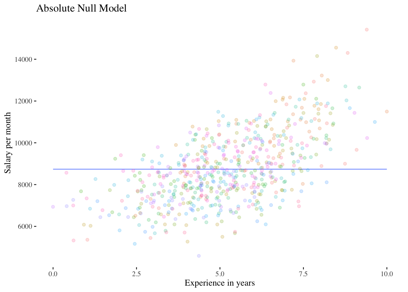
FALSE `geom_smooth()` using formula 'y ~ x'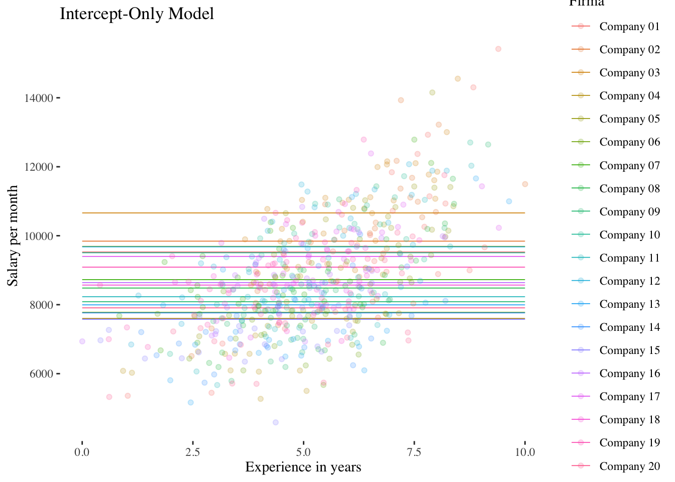
Shrinkage
We noted before that in an intercept-only-model the group intercepts “correspond” to the group means of salary. The estimated group means \((\hat\gamma_{00} + \upsilon_{0i})\) can be obtained with coef(). Let’s compare them to the empirical average salaries per company:
est_means <- coef(intercept.only.model)$company[,1]
emp_means <- df %>%
  group_by(company) %>%
  summarise(emp_means = mean(salary)) %>%
  ungroup() %>%
  dplyr::select(emp_means)

salary  <- tibble(est_means, emp_means) %>%
  mutate(diff_means = est_means - emp_means)

salary
## # A tibble: 20 × 3
## est_means emp_means diff_means
## <dbl> <dbl> <dbl>
## 1 9527. 9588. -60.4
## 2 9843. 9927. -84.6
## 3 10661. 10808. -147.
## 4 7601. 7514. 87.0
## 5 9691. 9764. -73.0
## 6 7779. 7705. 73.4
## 7 8727. 8727. 0.777
## 8 8483. 8463. 19.5
## 9 8086. 8036. 49.9
## 10 9506. 9565. -58.8
## 11 8231. 8193. 38.8
## 12 9678. 9750. -72.0
## 13 7995. 7938. 56.9
## 14 7762. 7687. 74.7
## 15 7576. 7487. 88.9
## 16 8640. 8632. 7.48
## 17 9400. 9450. -50.7
## 18 8569. 8557. 12.9
## 19 9089. 9116. -26.9
## 20 7908. 7844. 63.5We can see that the estimated intercepts are not equal to the actual empirical group means. In a multilevel model these estimates are obtained with “shrinkage”, i.e. they are “pulled” in the direction of the overall mean. This is because the level-2-residuals are assumed to be normally distributed and the uncertainty in the empirical estimates is accounted for in the sense that the company mean values of salary are corrected by weighting (“pooling”) them with the overall mean to arrive at the estimate \(\beta_{0i}=\hat\gamma_{00} + \upsilon_{0i}\).
This is also why multilevel models are sometimes called “partial-pooling models” (Gelman & Hill, 2011) as opposed to “no-pooling models” (linear models with groups as fixed effects without any assumptions regarding the level-2 variance).
Let’s look at such a “no-pooling model” for comparison:
no.pooling <- lm(salary ~ company, data = df)
summary(no.pooling)
##
## Call:
## lm(formula = salary ~ company, data = df)
##
## Residuals:
## Min 1Q Median 3Q Max
## -4229.1 -891.8 -40.1 779.5 5830.0
##
## Coefficients:
## Estimate Std. Error t value Pr(>|t|)
## (Intercept) 9587.70 255.26 37.560 < 2e-16 ***
## companyCompany 02 339.50 360.99 0.940 0.347369
## companyCompany 03 1220.13 360.99 3.380 0.000774 ***
## companyCompany 04 -2073.59 360.99 -5.744 1.49e-08 ***
## companyCompany 05 176.44 360.99 0.489 0.625201
## companyCompany 06 -1882.43 360.99 -5.215 2.57e-07 ***
## companyCompany 07 -861.02 360.99 -2.385 0.017393 *
## companyCompany 08 -1124.44 360.99 -3.115 0.001931 **
## companyCompany 09 -1551.27 360.99 -4.297 2.03e-05 ***
## companyCompany 10 -22.79 360.99 -0.063 0.949687
## companyCompany 11 -1395.12 360.99 -3.865 0.000124 ***
## companyCompany 12 162.29 360.99 0.450 0.653188
## companyCompany 13 -1649.80 360.99 -4.570 5.96e-06 ***
## companyCompany 14 -1900.22 360.99 -5.264 1.99e-07 ***
## companyCompany 15 -2100.36 360.99 -5.818 9.84e-09 ***
## companyCompany 16 -955.25 360.99 -2.646 0.008362 **
## companyCompany 17 -137.47 360.99 -0.381 0.703488
## companyCompany 18 -1031.08 360.99 -2.856 0.004441 **
## companyCompany 19 -471.97 360.99 -1.307 0.191585
## companyCompany 20 -1743.49 360.99 -4.830 1.75e-06 ***
## ---
## Signif. codes: 0 '***' 0.001 '**' 0.01 '*' 0.05 '.' 0.1 ' ' 1
##
## Residual standard error: 1398 on 580 degrees of freedom
## Multiple R-squared: 0.3154, Adjusted R-squared: 0.293
## F-statistic: 14.06 on 19 and 580 DF, p-value: < 2.2e-16The no-pooling model is equivalent to an ANOVA model, and the effects compare the salary means of Companies 02-20 with that of Company 01 (i.e. effects of dummy-coded variables with Company 01 as reference category). The \(R^2\) of the fixed effects model is slightly higher than the intraclass correlation from the intercept-only model (0.3154 vs. 0.3034), reflecting shrinkage in the multilevel model.
To get a model with estimates for all company means we can leave out the intercept:
no.pooling2 <- lm(salary ~ company - 1, data = df)
summary(no.pooling2)
##
## Call:
## lm(formula = salary ~ company - 1, data = df)
##
## Residuals:
## Min 1Q Median 3Q Max
## -4229.1 -891.8 -40.1 779.5 5830.0
##
## Coefficients:
## Estimate Std. Error t value Pr(>|t|)
## companyCompany 01 9587.7 255.3 37.56 <2e-16 ***
## companyCompany 02 9927.2 255.3 38.89 <2e-16 ***
## companyCompany 03 10807.8 255.3 42.34 <2e-16 ***
## companyCompany 04 7514.1 255.3 29.44 <2e-16 ***
## companyCompany 05 9764.1 255.3 38.25 <2e-16 ***
## companyCompany 06 7705.3 255.3 30.19 <2e-16 ***
## companyCompany 07 8726.7 255.3 34.19 <2e-16 ***
## companyCompany 08 8463.3 255.3 33.16 <2e-16 ***
## companyCompany 09 8036.4 255.3 31.48 <2e-16 ***
## companyCompany 10 9564.9 255.3 37.47 <2e-16 ***
## companyCompany 11 8192.6 255.3 32.09 <2e-16 ***
## companyCompany 12 9750.0 255.3 38.20 <2e-16 ***
## companyCompany 13 7937.9 255.3 31.10 <2e-16 ***
## companyCompany 14 7687.5 255.3 30.12 <2e-16 ***
## companyCompany 15 7487.3 255.3 29.33 <2e-16 ***
## companyCompany 16 8632.4 255.3 33.82 <2e-16 ***
## companyCompany 17 9450.2 255.3 37.02 <2e-16 ***
## companyCompany 18 8556.6 255.3 33.52 <2e-16 ***
## companyCompany 19 9115.7 255.3 35.71 <2e-16 ***
## companyCompany 20 7844.2 255.3 30.73 <2e-16 ***
## ---
## Signif. codes: 0 '***' 0.001 '**' 0.01 '*' 0.05 '.' 0.1 ' ' 1
##
## Residual standard error: 1398 on 580 degrees of freedom
## Multiple R-squared: 0.9761, Adjusted R-squared: 0.9753
## F-statistic: 1185 on 20 and 580 DF, p-value: < 2.2e-16The F statistic of this model now also includes the test of the group means against 0, thus we would not use it for the purpose of comparing salary means across companies.
Let’s check whether the estimates of this model are really equal to the group means:
# extract "no-pooling" means from model no.pooling2
np_means <- as.numeric(coef(no.pooling2))
# strip emp-means of unneeded attributes
emp_means <- as.numeric(unlist(emp_means))
# check equivalence
all.equal(np_means, emp_means)
## [1] TRUEFinally, let’s plot the estimated means from the multilevel (“partial-pooling”) intercept-only model and those from the linear (“no-pooling”) model (empirical company means):
salary %>% pivot_longer(-diff_means, names_to = "means", values_to = "salary") %>%
  mutate(means = as.factor(means)) %>%
  ggplot(aes(x = means, y = salary)) +
  geom_boxplot(aes(color = means)) +
  geom_point(alpha = 0.6) +
  guides(color = "none") +
  scale_color_brewer(palette = "Set1") +
  theme_classic()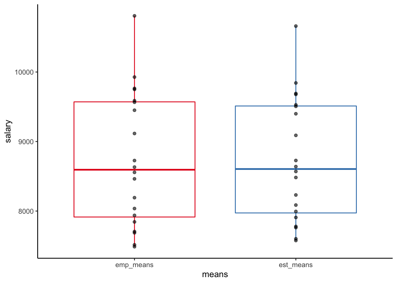
We can see that the distribution of the empirical means is slightly broader than that of the estimated (“shrunken”) means. In case of unequal company sample sizes shrinkage would be more pronounced, with means from companies with smaller samples more “pulled” to the overall mean than means from companies with large samples, reflecting the lower precision of estimates coming from small samples.
10.2.2 Random-Intercept-Model (Model 2)
This model contains a level-1 predictor (experience), but it is conceptualized as a fixed effect (no random slope, only random intercept). This model is particularly useful to determine the proportion of variance explained by the level-1 predictor and as a comparison model for testing the random slope in the Random-Coefficients-Model (see below Model 3).
Level-1 model:
\(\boldsymbol {y_{mi}=\beta_{0i} + \beta_{1i} \cdot x_{mi} + \epsilon_{mi}}\)
Level-2 model:
\(\boldsymbol {\beta_{0i}=\gamma_{00} + \upsilon_{0i}}\)
\(\boldsymbol {\beta_{1i}=\gamma_{10}}\)
Overall model:
\(\boldsymbol {y_{mi}=\gamma_{00} + \gamma_{10} \cdot x_{mi} + \upsilon_{0i}+\epsilon_{mi}}\)
Estimating the model
random.intercept.model <-  lmer(salary ~ experience + (1 | company),
                                data = df, REML = TRUE)

df$random.intercept.preds <-  predict(random.intercept.model)

summary(random.intercept.model)
## Linear mixed model fit by REML. t-tests use Satterthwaite's method [
## lmerModLmerTest]
## Formula: salary ~ experience + (1 | company)
## Data: df
##
## REML criterion at convergence: 10127.1
##
## Scaled residuals:
## Min 1Q Median 3Q Max
## -2.8109 -0.6884 0.0005 0.5980 3.8833
##
## Random effects:
## Groups Name Variance Std.Dev.
## company (Intercept) 614367 783.8
## Residual 1184502 1088.3
## Number of obs: 600, groups: company, 20
##
## Fixed effects:
## Estimate Std. Error df t value Pr(>|t|)
## (Intercept) 5964.18 229.41 48.00 26.00 <2e-16 ***
## experience 534.34 27.21 589.48 19.64 <2e-16 ***
## ---
## Signif. codes: 0 '***' 0.001 '**' 0.01 '*' 0.05 '.' 0.1 ' ' 1
##
## Correlation of Fixed Effects:
## (Intr)
## experience -0.615The results show that the fixed effect of experience is positively significant \((\hat\gamma_{10} = 534.34, p < 0.001)\). Across all companies, the predicted income thus increases with each year of experience by about 534 units (e.g. CHF).
Explanation of variance by a level-1 predictor
How much level-1 variance is explained by experience?
\(R^2_{Level-1} = \frac {\sigma^2_{\epsilon_1} - \sigma^2_{\epsilon_2}}{\sigma^2_{\epsilon_1}} = \frac {{1954745}-{1184502}}{1954745} = {0.394}\)
Let us look at the output of summ() for this model:
summ(random.intercept.model)## MODEL INFO:
## Observations: 600
## Dependent Variable: salary
## Type: Mixed effects linear regression
##
## MODEL FIT:
## AIC = 10135.09, BIC = 10152.68
## Pseudo-R² (fixed effects) = 0.33
## Pseudo-R² (total) = 0.56
##
## FIXED EFFECTS:
## -------------------------------------------------------------
## Est. S.E. t val. d.f. p
## ----------------- --------- -------- -------- -------- ------
## (Intercept) 5964.18 229.41 26.00 48.00 0.00
## experience 534.34 27.21 19.64 589.48 0.00
## -------------------------------------------------------------
##
## p values calculated using Satterthwaite d.f.
##
## RANDOM EFFECTS:
## ------------------------------------
## Group Parameter Std. Dev.
## ---------- ------------- -----------
## company (Intercept) 783.82
## Residual 1088.35
## ------------------------------------
##
## Grouping variables:
## ---------------------------
## Group # groups ICC
## --------- ---------- ------
## company 20 0.34
## ---------------------------summ() includes Pseudo-R^2 (fixed effects) and Pseudo-R^2 (total) (also called “marginal” and “conditional”). Pseudo-R^2 (fixed effects) represents the proportion of (overall) variance explained by the predictors (fixed effects), while Pseudo-R^2 (total) represents a measure of the total variance explained by the fixed effects + the variance that can be attributed to the random effects (i.e. are represented by the random variance(s)).
## `geom_smooth()` using formula 'y ~ x'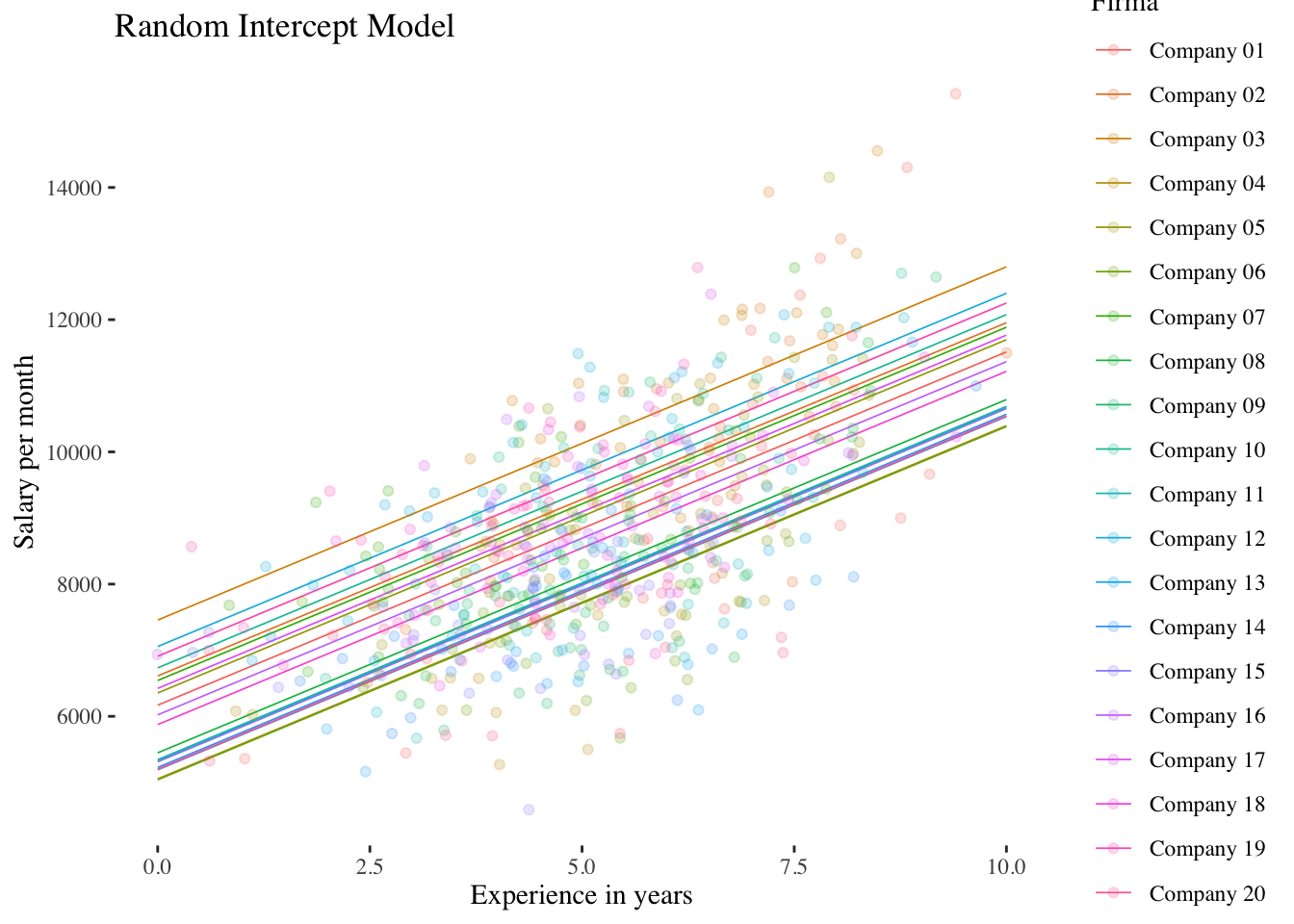
10.2.3 Random-Coefficients-Model (Model 3)
This model contains both a random intercept and a random slope. Applying this model, the (random) variance of the slope of the level-1 predictor can be estimated. This gives us a measure of the differences in the effect (slope) of the level-1 predictor experience on salary between the level-2 units (companies).
Level-1 model:
\(\boldsymbol {y_{mi}=\beta_{0i} + \beta_{1i} \cdot x_{mi} + \epsilon_{mi}}\)
Level-2 model:
\(\boldsymbol {\beta_{0i}=\gamma_{00} + \upsilon_{0i}}\)
\(\boldsymbol {\beta_{1i}=\gamma_{10} + \upsilon_{1i}}\)
Overall model:
\(\boldsymbol {y_{mi}=\gamma_{00} + \gamma_{10} \cdot x_{mi} + \upsilon_{0i} + \upsilon_{1i} \cdot x_{mi} + \epsilon_{mi}}\)
Estimating the model
random.coefficients.model <-  lmer(salary ~ experience + (experience | company),
                                   data = df, REML = TRUE)

df$random.coefficients.preds <-  predict(random.coefficients.model)

summary(random.coefficients.model)
## Linear mixed model fit by REML. t-tests use Satterthwaite's method [
## lmerModLmerTest]
## Formula: salary ~ experience + (experience | company)
## Data: df
##
## REML criterion at convergence: 10117.1
##
## Scaled residuals:
## Min 1Q Median 3Q Max
## -2.8308 -0.6804 0.0037 0.5999 3.3607
##
## Random effects:
## Groups Name Variance Std.Dev. Corr
## company (Intercept) 722929 850.3
## experience 18398 135.6 -0.51
## Residual 1136284 1066.0
## Number of obs: 600, groups: company, 20
##
## Fixed effects:
## Estimate Std. Error df t value Pr(>|t|)
## (Intercept) 5933.70 240.41 18.88 24.68 7.86e-16 ***
## experience 530.85 40.59 18.94 13.08 6.23e-11 ***
## ---
## Signif. codes: 0 '***' 0.001 '**' 0.01 '*' 0.05 '.' 0.1 ' ' 1
##
## Correlation of Fixed Effects:
## (Intr)
## experience -0.690The results show that the fixed effect of experience is again positively significant \((\hat\gamma_{10} = 530.85, p < 0.001)\). However, our main interest with regard to the random coefficients model is the variance/standard deviation of the random slope: \(\hat\sigma^2_{\upsilon_1} = 18398\) and thus \(\hat\sigma_{\upsilon_1} = \sqrt{18398} = 135.6\). The average deviation (level-2 residual \(\upsilon_{1i}\)) of the experience effect of a company from the average effect \(\hat\gamma_{10}\) is therefore about 136 units (e.g. CHF).
With ranef() we can again get the individual random effects (now level-2 residuals of the intercept \(\upsilon_{0i}\) plus those of the slope \(\upsilon_{1i}\)):
ranef(random.coefficients.model)## $company
## (Intercept) experience
## Company 01 -1004.039997 203.783949
## Company 02 -160.905460 143.414219
## Company 03 705.225696 139.872130
## Company 04 -611.893521 -54.004725
## Company 05 -34.012184 76.647610
## Company 06 -123.862139 -150.710472
## Company 07 669.605902 -13.637058
## Company 08 -830.957427 65.842873
## Company 09 -1020.972535 86.048006
## Company 10 392.990609 81.956356
## Company 11 -769.218300 37.972728
## Company 12 1249.053517 -25.058149
## Company 13 -593.441952 -25.439847
## Company 14 -186.173090 -109.528639
## Company 15 7.274997 -150.172232
## Company 16 773.002541 -140.843276
## Company 17 562.157337 -11.057795
## Company 18 508.311643 -112.496132
## Company 19 1006.299627 -6.703797
## Company 20 -538.445264 -35.885749
##
## with conditional variances for "company"The output also contains information about the third random effect parameter estimated in this model: the covariance \(\hat\sigma_{\upsilon_0\upsilon_1}\) between the level-2 residuals of the intercept and the level-2 residuals of the slope. However, it is not the covariance itself that is shown, but the correlation \(r_{\upsilon_0\upsilon_1} = -0.51\). Thus, the average salary of an entry-level employee in a company (predicted value of salary at experience = 0) is negatively correlated with the slope of experience: In companies where newly hired employees already earn well, there seems to be less room for salary increases than in companies with lower starting salaries.
Significance test for \(\sigma^2_{\upsilon_1}\): Comparisons with the random intercept model
If we compare this model to the random intercept model using an LR-test, two parameters are tested simultaneously: the level-2 variance of the slope (\(\sigma^2_{\upsilon_1}\)) and the level-2 covariance/correlation between intercept and slope (\(\sigma_{\upsilon0\upsilon1}\)).
The model comparison can again be carried out using ranova():
ranova(random.coefficients.model)## ANOVA-like table for random-effects: Single term deletions
##
## Model:
## salary ~ experience + (experience | company)
## npar logLik AIC LRT Df Pr(>Chisq)
## <none> 6 -5058.5 10129
## experience in (experience | company) 4 -5063.5 10135 10.011 2 0.006699 **
## ---
## Signif. codes: 0 '***' 0.001 '**' 0.01 '*' 0.05 '.' 0.1 ' ' 1Alternatively, we can perform the model comparison using anova() by explicitly specifying both models:
anova(random.coefficients.model, random.intercept.model, refit = FALSE)## Data: df
## Models:
## random.intercept.model: salary ~ experience + (1 | company)
## random.coefficients.model: salary ~ experience + (experience | company)
## npar AIC BIC logLik deviance Chisq Df
## random.intercept.model 4 10135 10153 -5063.5 10127
## random.coefficients.model 6 10129 10156 -5058.5 10117 10.011 2
## Pr(>Chisq)
## random.intercept.model
## random.coefficients.model 0.006699 **
## ---
## Signif. codes: 0 '***' 0.001 '**' 0.01 '*' 0.05 '.' 0.1 ' ' 1With anova(), in the default setting (refit = TRUE) both models are automatically estimated again (refitted) using ML (instead of REML) before performing the LR test in case REML was used before as estimation method. This is a precautionary measure taken by the developers in order to avoid the common mistake of comparing REML-estimated models, which (also) differ in their fixed effects structure. Since here we are comparing two models that differ only in their random effects structure, we choose refit = FALSE to get the comparison of the REML-fitted models. This issue is not relevant for model comparisons using ranova(), since here a model fitted with REML or ML is automatically compared with the corresponding reduced model. Thus, since ranova() only performs model comparisons to test random effects the refit problem does not exist there.
The results show a significant LR test, thus the set of two parameters is significantly different from 0, but the p-value is not quite correct, since one of the two parameters - \(\sigma^2_{\upsilon_1}\) - has a bounded parameter space (cannot become < 0). The correct p-value is therefore even smaller than the one given in the output: the correct test distribution is a mixture distribution of \(\chi^2_{df=1}\) and \(\chi^2_{df=2}\). The critical chi-square value of this mixture distribution is 5.14 (Snijders & Bosker, 2012).
The exact computation of the p-value based on the mixture distribution is done by averaging the p-values of the two distributions with \(df = 1\) and \(df = 2\):
0.5 * pchisq(10.011, 1, lower.tail = FALSE) +
  0.5 * pchisq(10.011, 2, lower.tail = FALSE)
## [1] 0.004128535\(~\)
## `geom_smooth()` using formula 'y ~ x'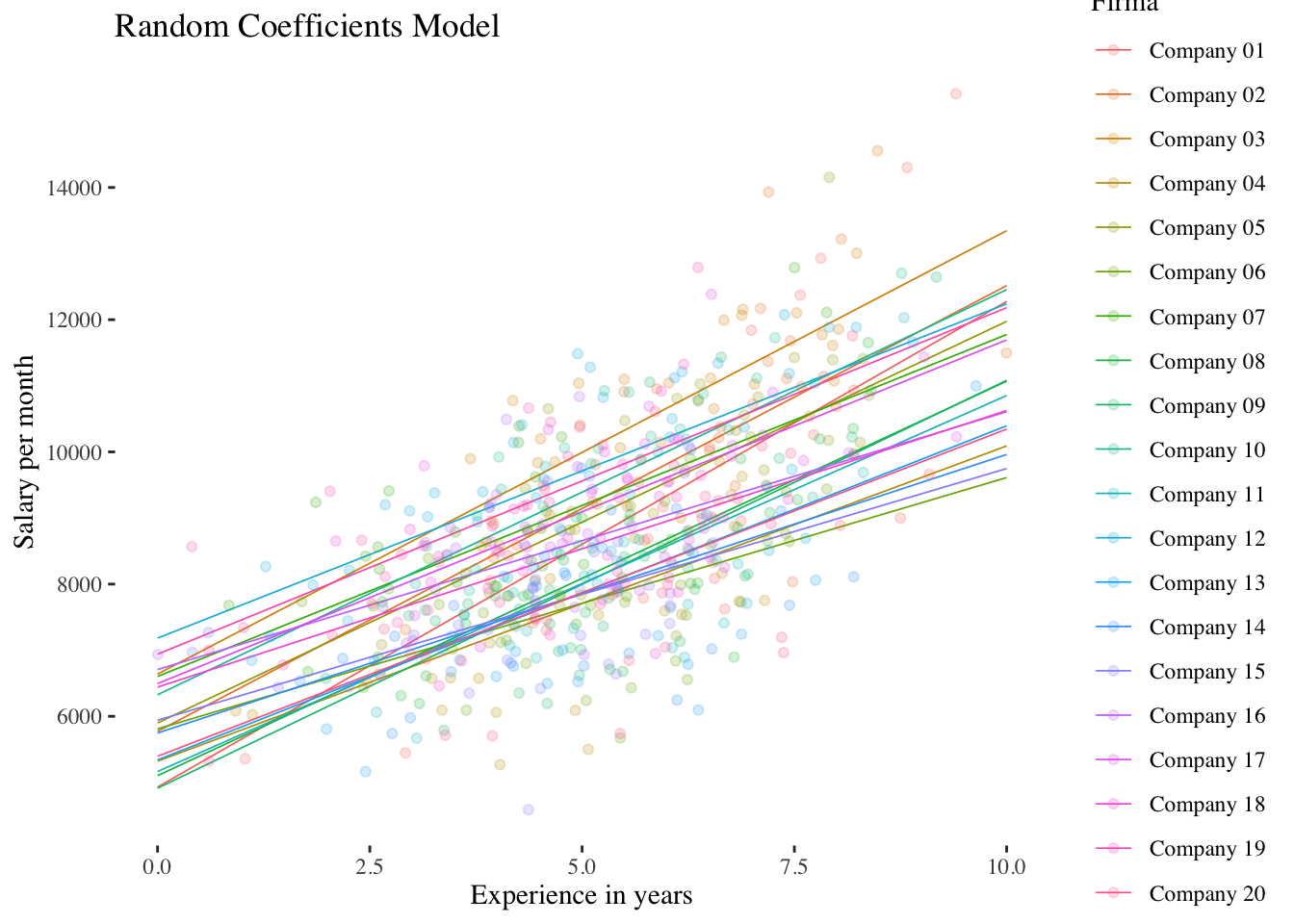
Shrinkage
The shrinkage logic also applies to the random slopes: let’s compare the multilevel “partial-pooling” Random-Coefficients-Model to the fixed effects “no-pooling” linear model where the company differences in the slope of experience are represented by an interaction effect with the company factor:
no.pooling3 <- lm(salary ~ company*experience, data = df)
summary(no.pooling3)
##
## Call:
## lm(formula = salary ~ company * experience, data = df)
##
## Residuals:
## Min 1Q Median 3Q Max
## -2975.7 -686.6 -8.7 666.1 3357.7
##
## Coefficients:
## Estimate Std. Error t value Pr(>|t|)
## (Intercept) 4045.51 674.47 5.998 3.59e-09 ***
## companyCompany 02 1230.86 1004.50 1.225 0.220960
## companyCompany 03 2515.51 1099.24 2.288 0.022486 *
## companyCompany 04 1272.21 910.62 1.397 0.162946
## companyCompany 05 1564.32 1074.58 1.456 0.146021
## companyCompany 06 2187.88 941.93 2.323 0.020549 *
## companyCompany 07 2703.24 856.65 3.156 0.001688 **
## companyCompany 08 430.44 1003.40 0.429 0.668105
## companyCompany 09 75.61 1004.33 0.075 0.940014
## companyCompany 10 2171.04 949.49 2.287 0.022595 *
## companyCompany 11 593.45 1020.74 0.581 0.561208
## companyCompany 12 3440.03 839.83 4.096 4.82e-05 ***
## companyCompany 13 1171.11 910.85 1.286 0.199069
## companyCompany 14 1935.09 882.47 2.193 0.028731 *
## companyCompany 15 2333.85 872.03 2.676 0.007661 **
## companyCompany 16 3276.02 909.29 3.603 0.000343 ***
## companyCompany 17 2786.10 1028.06 2.710 0.006933 **
## companyCompany 18 3125.47 1019.61 3.065 0.002279 **
## companyCompany 19 3060.14 837.38 3.654 0.000282 ***
## companyCompany 20 1286.92 881.36 1.460 0.144810
## experience 869.45 101.31 8.582 < 2e-16 ***
## companyCompany 02:experience -110.71 154.93 -0.715 0.475147
## companyCompany 03:experience -172.46 171.86 -1.003 0.316074
## companyCompany 04:experience -403.59 159.37 -2.532 0.011600 *
## companyCompany 05:experience -213.82 163.55 -1.307 0.191629
## companyCompany 06:experience -580.85 159.46 -3.643 0.000295 ***
## companyCompany 07:experience -377.35 158.69 -2.378 0.017748 *
## companyCompany 08:experience -170.62 161.41 -1.057 0.290930
## companyCompany 09:experience -109.10 172.39 -0.633 0.527074
## companyCompany 10:experience -226.53 159.16 -1.423 0.155217
## companyCompany 11:experience -211.90 170.48 -1.243 0.214397
## companyCompany 12:experience -408.39 138.11 -2.957 0.003237 **
## companyCompany 13:experience -349.60 150.19 -2.328 0.020281 *
## companyCompany 14:experience -505.93 152.42 -3.319 0.000961 ***
## companyCompany 15:experience -602.54 160.61 -3.752 0.000194 ***
## companyCompany 16:experience -600.79 155.86 -3.855 0.000129 ***
## companyCompany 17:experience -402.81 167.86 -2.400 0.016732 *
## companyCompany 18:experience -593.96 178.54 -3.327 0.000936 ***
## companyCompany 19:experience -369.10 152.23 -2.425 0.015642 *
## companyCompany 20:experience -371.25 146.41 -2.536 0.011493 *
## ---
## Signif. codes: 0 '***' 0.001 '**' 0.01 '*' 0.05 '.' 0.1 ' ' 1
##
## Residual standard error: 1066 on 560 degrees of freedom
## Multiple R-squared: 0.6156, Adjusted R-squared: 0.5888
## F-statistic: 22.99 on 39 and 560 DF, p-value: < 2.2e-16A significance test for the overall fixed effects slope differences (overall interaction effect) is obtained by comparing with a main effects model:
no.pooling3a <- lm(salary ~ company + experience, data = df)
anova(no.pooling3a, no.pooling3)
## Analysis of Variance Table
##
## Model 1: salary ~ company + experience
## Model 2: salary ~ company * experience
## Res.Df RSS Df Sum of Sq F Pr(>F)
## 1 579 685829891
## 2 560 636629138 19 49200753 2.2778 0.001607 **
## ---
## Signif. codes: 0 '***' 0.001 '**' 0.01 '*' 0.05 '.' 0.1 ' ' 1The p-value (p = 0.0016) of the interaction is even smaller than the one for the slope variance of Model 3 above (p = 0.0041), reflecting the no-pooling approach of the fixed-effects linear model.
Let’s compare the experience slopes of the fixed-effects versus the multilevel random coefficients model also graphically:
# extract fixed slopes from the no.pooling3 model
fixed_slopes <- as.numeric(c(coef(no.pooling3)[21], coef(no.pooling3)[21] + coef(no.pooling3)[22:40]))
# extract random slopes from the random.coefficients.model
random_slopes <- as.numeric(unlist(coef(random.coefficients.model)$company[2]))
# put them in a data frame
slopes <- tibble(fixed_slopes, random_slopes)

# pivot the data frame and plot
slopes %>% pivot_longer(everything(), names_to = "slopes", values_to = "b") %>%
  mutate(slopes = as.factor(slopes)) %>%
  ggplot(aes(x = slopes, y = b)) +
  geom_boxplot(aes(color = slopes)) +
  geom_point(alpha = 0.6) +
  guides(color = "none") +
  scale_color_brewer(palette = "Set1") +
  theme_classic()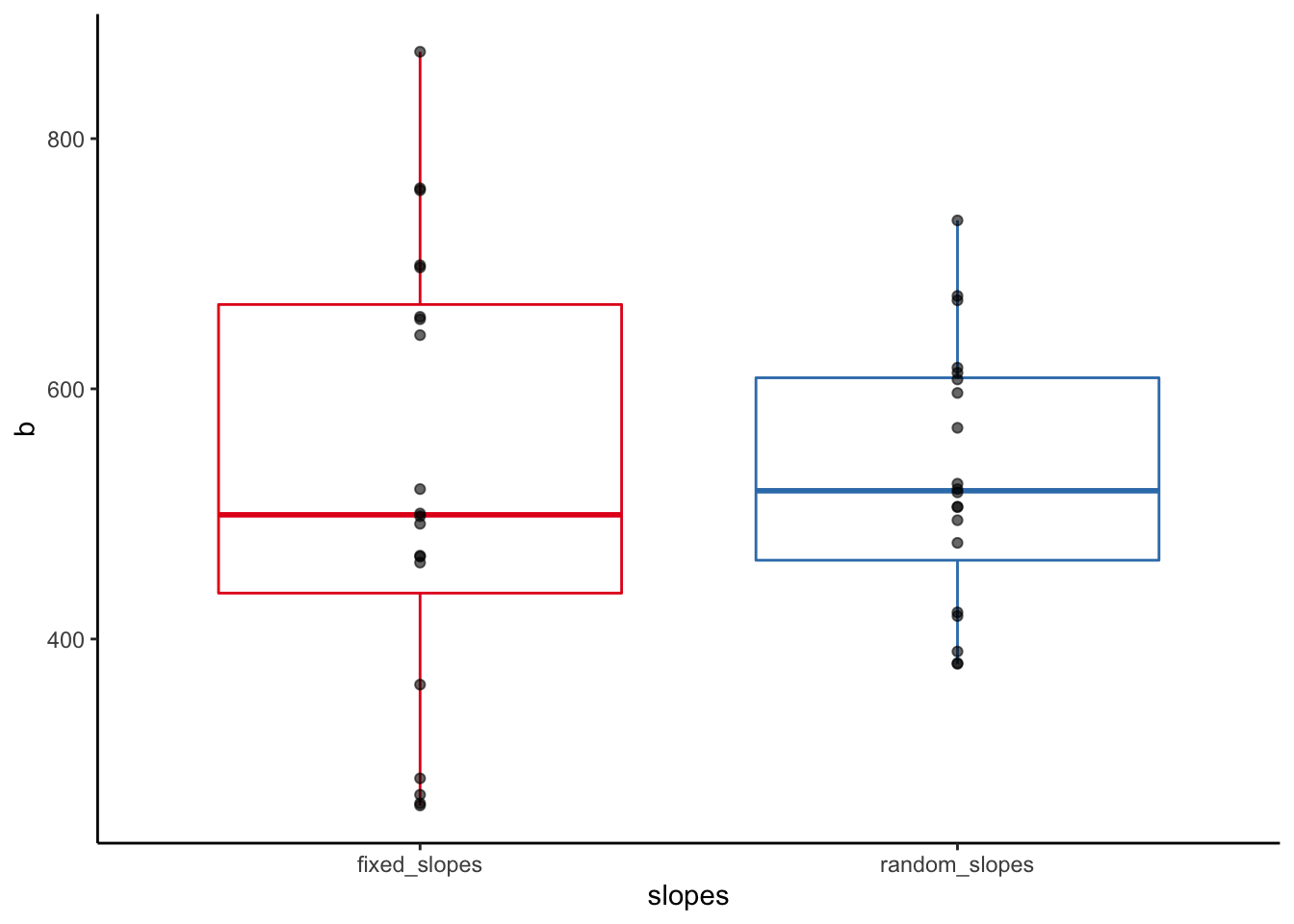
Shrinkage ist rather pronounced here!
10.2.4 ggplot2 code for the plots
# Definition of axis labels (for all plats)
xlabel <- "Experience in years"
ylabel <- "Salary per month"

# Intercept Only Model
intercept.only.graph <-  ggplot(data = df,
                                aes(x = experience,
                                    y = intercept.only.preds,
                                    colour = company)) +
    geom_smooth(method = "lm", fullrange = TRUE, size = 0.3) +
    geom_jitter(aes(x = experience, y = salary,
                    group = company, colour = company),
                alpha = 0.2) +
    labs(x = xlabel, y = ylabel) +
    ggtitle("Intercept Only Model") +
    scale_colour_discrete('Company') +
    theme_tufte()

# Random Intercept Model
random.intercept.graph <-  ggplot(data = df,
                                  aes(x = experience,
                                      y = random.intercept.preds,
                                      colour = company)) +
    geom_smooth(method = "lm", fullrange = TRUE, size = 0.3) +
    geom_jitter(aes(x = experience, y = salary, group = company, colour = company),
                alpha = 0.2) +
    labs(x = xlabel, y = ylabel) +
    ggtitle("Random Intercept Model") +
    scale_colour_discrete('Company') +
    theme_tufte()

# Random Coefficients Model
random.coefficients.graph <-  ggplot(data = df,
                                  aes(x = experience,
                                      y = random.coefficients.preds,
                                      colour = company)) +
    geom_smooth(method = "lm", fullrange = TRUE, size = 0.3) +
    geom_jitter(aes(x = experience, y = salary,
                    group = company, colour = company),
                alpha = 0.2) +
    labs(x = xlabel, y = ylabel) +
    ggtitle("Random Coefficients Model") +
    scale_colour_discrete('Company') +
    theme_tufte()
10.3 Models including level-2 predictors
10.3.1 Intercept-as-Outcome-Model (Model 4)
Context effect model
The context effect model is a variant of the (more general) intercept-as-outcome model where the level-2 predictor corresponds to a (group-)aggregated level-1 predictor (here: experience_gm; where "_gm" stands for group mean). To separate the effects of the level-1 and the level-2 predictor, the level-1 predictor has to be included as a group-centered variable. Thus, at level-1, only the individual deviation of experience from the respective company-specific experience_gm is modeled, the group-centered variable is therefore called experience_gc (with "_gc" standing for group-centered).
In our example, the level-2 predictor is thus the average experience per company. The effect of this variable is examined together with the group-centered experience. In addition to the assumption that individual experience is associated with a higher salary, we now additionally assume that the average experience of a company’s employees affects the average salary of a company. In this example, it is reasonable to assume that both effects are present and go in the same direction. But this is not always the case (compare for example the “Big-Fish-Little-Pond-Effect”).
In the context effect model, often no random slope of the level-1 predictor is included.
\(~\)
Level-1 model:
\(\boldsymbol {y_{mi}=\beta_{0i} + \beta_{1i} \cdot (x_{mi} - \mu_{\cdot i(X)}) + \epsilon_{mi}}\)
Level-2 model:
\(\boldsymbol {\beta_{0i}=\gamma_{00} + \gamma_{01} \cdot \mu_{\cdot i(X)} + \upsilon_{0i}}\)
\(\boldsymbol {\beta_{1i}=\gamma_{10}}\)
Overall model:
\(\boldsymbol {y_{mi}=\gamma_{00} + \gamma_{10} \cdot (x_{mi} - \mu_{\cdot i(X)}) + \gamma_{01} \cdot \mu_{\cdot i(X)} + \upsilon_{0i} + \epsilon_{mi}}\)
\(~\)
The level-2 predictor experience_gm needs to be calculated and assigned to each person first. We calculate this variable using group_by() and mutate() from the tidyverse package. Also, we calculate a group-centered variable experience_gc by subtracting for each person their respective company average from their individual experience value.
df <- df %>%
  group_by(company) %>%
  mutate(experience_gm = mean(experience),
         experience_gc = experience - experience_gm) %>%
  ungroup() %>%
  dplyr::select(company, sector, experience, experience_gm, experience_gc, salary)
# select() only changes the order of variables here

# Did everything work out fine?
head(df)
## # A tibble: 6 × 6
## company sector experience experience_gm experience_gc salary
## <fct> <fct> <dbl> <dbl> <dbl> <dbl>
## 1 Company 01 Private 6.87 6.37 0.496 8957.
## 2 Company 01 Private 5.66 6.37 -0.714 9545.
## 3 Company 01 Private 4.58 6.37 -1.79 7304.
## 4 Company 01 Private 6.56 6.37 0.186 8089.
## 5 Company 01 Private 8.83 6.37 2.46 14303.
## 6 Company 01 Private 7.73 6.37 1.36 10259.tail(df)## # A tibble: 6 × 6
## company sector experience experience_gm experience_gc salary
## <fct> <fct> <dbl> <dbl> <dbl> <dbl>
## 1 Company 20 Private 3.58 5.04 -1.46 6838.
## 2 Company 20 Private 3.18 5.04 -1.86 7604.
## 3 Company 20 Private 3.39 5.04 -1.65 5714.
## 4 Company 20 Private 7.12 5.04 2.08 10089.
## 5 Company 20 Private 2.98 5.04 -2.06 6940.
## 6 Company 20 Private 6.45 5.04 1.41 9330.# Let's also have a look at the company means of experience:
df %>%
group_by(company) %>%
summarise(experience_gm = mean(experience_gm)) %>%
ungroup()## # A tibble: 20 × 2
## company experience_gm
## <fct> <dbl>
## 1 Company 01 6.37
## 2 Company 02 6.13
## 3 Company 03 6.09
## 4 Company 04 4.71
## 5 Company 05 6.34
## 6 Company 06 5.1
## 7 Company 07 4.02
## 8 Company 08 5.71
## 9 Company 09 5.15
## 10 Company 10 5.21
## 11 Company 11 5.40
## 12 Company 12 4.91
## 13 Company 13 5.23
## 14 Company 14 4.70
## 15 Company 15 4.15
## 16 Company 16 4.88
## 17 Company 17 5.61
## 18 Company 18 5.03
## 19 Company 19 4.02
## 20 Company 20 5.04Estimating the model
context.model <- lmer(salary ~ experience_gc + experience_gm + (1 | company),
                      data = df, REML = TRUE)

df$context.model.preds <- predict(context.model)

summary(context.model)
## Linear mixed model fit by REML. t-tests use Satterthwaite's method [
## lmerModLmerTest]
## Formula: salary ~ experience_gc + experience_gm + (1 | company)
## Data: df
##
## REML criterion at convergence: 10113.3
##
## Scaled residuals:
## Min 1Q Median 3Q Max
## -2.7991 -0.6796 0.0043 0.6008 3.8752
##
## Random effects:
## Groups Name Variance Std.Dev.
## company (Intercept) 622987 789.3
## Residual 1184508 1088.4
## Number of obs: 600, groups: company, 20
##
## Fixed effects:
## Estimate Std. Error df t value Pr(>|t|)
## (Intercept) 4779.25 1387.36 18.00 3.445 0.00289 **
## experience_gc 531.88 27.35 579.00 19.446 < 2e-16 ***
## experience_gm 762.64 264.99 18.00 2.878 0.01001 *
## ---
## Signif. codes: 0 '***' 0.001 '**' 0.01 '*' 0.05 '.' 0.1 ' ' 1
##
## Correlation of Fixed Effects:
## (Intr) exprnc_gc
## experinc_gc 0.000
## experinc_gm -0.991 0.000The effect of experience_gc is very similar to the corresponding effect in the random intercept model. The effect of experience_gm is more than twice as large - every year of (average) experience that the employees of one company can look back to more than the employees of another company increases the predicted salary of the employees of that company (and thus the intercept \(\hat\beta_{0i}\)) by \(\hat\gamma_{01} = 762.64\) CHF.
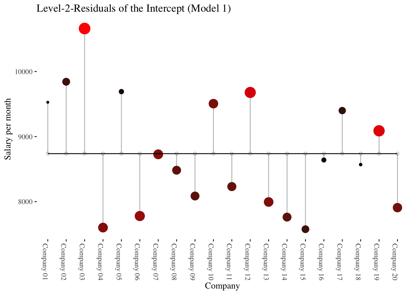
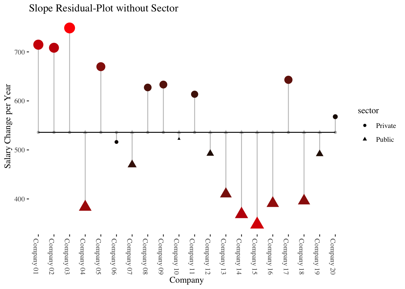
The following plots illustrate data at the company level (level-2) only.
The first plot shows the deviations (level-2 residuals \(\upsilon_{0i}\)) of the individual company intercepts from the total mean of the intercepts (\(\hat\gamma_{00}\)) in the intercept-only-model.
The average salaries of the companies differ greatly from the average salary across all companies.
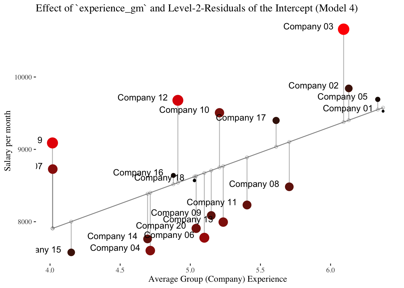
In the second plot, the level-2 predictor experience_gm comes into play.
It is shown that experience_gm differs between the companies and that it correlates positively with the intercepts of the intercept-only-model (linear slope = \(\hat\gamma_{01} = 762.64\)).
General Intercept-as-Outcome Model
This is a model including a main effect of a level-2 predictor (prediction of the intercept), with a random intercept, and with or without a random slope. In this model we examine to what extent the sector in which the firms operate has an effect on salary, i.e. whether the salary depends on the sector in which a company operates (private or public).
The effect of a level-2 predictor could also be determined without any other (level-1) predictors in the model. As in our case, however, one often would like to know what effect a level-2 predictor has in the context of a specific level-1 predictor present. In this model, the level-1 predictor can be modeled either including a random slope (\(\beta_{1i}=\gamma_{10} + \upsilon_{1i}\)) or not including a random slope (\(\beta_{1i}=\gamma_{10}\)) (the difference is similar to the difference between the random coefficients model and the random intercept model).
Here, we will only look at an intercept-as-outcome model including a random-slope of the level-1 predictor.
\(~\)
Level-1 model:
\(\boldsymbol {y_{mi}=\beta_{0i} + \beta_{1i} \cdot x_{mi} + \epsilon_{mi}}\)
Level-2 model:
\(\boldsymbol {\beta_{0i}=\gamma_{00} + \gamma_{01} \cdot z_i + \upsilon_{0i}}\)
\(\boldsymbol {\beta_{1i}=\gamma_{10} + \upsilon_{1i}}\)
Overall model:
\(\boldsymbol {y_{mi}=\gamma_{00} + \gamma_{10} \cdot x_{mi} + \gamma_{01} \cdot z_i + \upsilon_{0i} \cdot x_{mi} + \epsilon_{mi}}\)
\(~\)
Estimating the model
In contrast to the variable experience_gm (level-2 predictor in the context effect model), sector is a categorical variable (factor).
Conveniently, lme4 does the dummy coding (with the first factor level Private as reference category) for us.
intercept.as.outcome.model <- lmer(salary ~ experience + sector +
                                     (experience | company),
                                   data = df, REML = TRUE)

df$intercept.as.outcome.preds <- predict(intercept.as.outcome.model)

summary(intercept.as.outcome.model)
## Linear mixed model fit by REML. t-tests use Satterthwaite's method [
## lmerModLmerTest]
## Formula: salary ~ experience + sector + (experience | company)
## Data: df
##
## REML criterion at convergence: 10102.1
##
## Scaled residuals:
## Min 1Q Median 3Q Max
## -2.8397 -0.6713 0.0018 0.6041 3.3846
##
## Random effects:
## Groups Name Variance Std.Dev. Corr
## company (Intercept) 487110 697.9
## experience 18614 136.4 -0.31
## Residual 1136311 1066.0
## Number of obs: 600, groups: company, 20
##
## Fixed effects:
## Estimate Std. Error df t value Pr(>|t|)
## (Intercept) 5657.87 285.68 24.12 19.805 < 2e-16 ***
## experience 532.42 40.77 19.06 13.060 5.86e-11 ***
## sectorPublic 529.51 343.42 18.15 1.542 0.14
## ---
## Signif. codes: 0 '***' 0.001 '**' 0.01 '*' 0.05 '.' 0.1 ' ' 1
##
## Correlation of Fixed Effects:
## (Intr) exprnc
## experience -0.491
## sectorPublc -0.662 0.062Employees in the public sector earn about 529 CHF more than employees in the private sector (\(\hat\gamma_{01} =\) 529.51), but this effect is not significant (\(p =\) 0.14). The interpretation of the \(\hat\gamma_{00} =\) 5657.87 has also changed. Now it refers to the average monthly salary for an employee of an (unknown) company in the private sector (reference category) who does not have any work experience (experience = 0). Such a person earns about 5658 CHF.
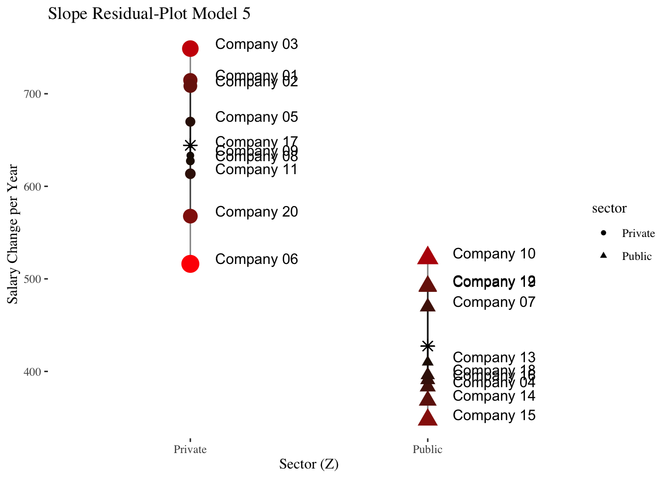
10.3.2 Slope-as-Outcome-Model (Model 5)
In this model we ask whether the (significant) level-2 variance of the slope of experience (\(\hat\sigma_{\upsilon_1}^2\)) found in Model 3 depends on the level-2 predictor sector. Thus, do the (level-2 residuals of the) slopes of experience differ between companies from the public and the private sector?
It could be that salary increases are stronger in the private as compared to the public sector, where salary increases are weaker and largely based on seniority.
Note: Strictly speaking, now, model 4 is the comparison model (and not model 3) because it contains (like model 5) the level-2 main effect of sector. But conceptually we ask whether the significant slope variance from the random coefficients model is reduced when considering the sector a company operates in.
\(~\)
level-1 model:
\(\boldsymbol {y_{mi}=\beta_{0i} + \beta_{1i} \cdot x_{mi} + \epsilon_{mi}}\)
level-2 model:
\(\boldsymbol {\beta_{0i}=\gamma_{00} + \gamma_{01} \cdot z_i + \upsilon_{0i}}\)
\(\boldsymbol {\beta_{1i}=\gamma_{10} + \gamma_{11} \cdot z_i + \upsilon_{1i}}\)
Overall model:
\(\boldsymbol {y_{mi}=\gamma_{00} + \gamma_{10} \cdot x_{mi} + \gamma_{01} \cdot z_i + \gamma_{11} \cdot x_{mi} \cdot z_i + \upsilon_{0i} + \upsilon_{1i} \cdot x_{mi} + \epsilon_{mi}}\)
\(~\)
Estimating the model
slope.as.outcome.model <- lmer(salary ~ experience*sector +
                         (experience | company),
                         data = df, REML = TRUE)

summary(slope.as.outcome.model)
## Linear mixed model fit by REML. t-tests use Satterthwaite's method [
## lmerModLmerTest]
## Formula: salary ~ experience * sector + (experience | company)
## Data: df
##
## REML criterion at convergence: 10083.1
##
## Scaled residuals:
## Min 1Q Median 3Q Max
## -2.8271 -0.6923 -0.0319 0.6088 3.4093
##
## Random effects:
## Groups Name Variance Std.Dev. Corr
## company (Intercept) 341720 584.57
## experience 7713 87.82 0.13
## Residual 1137612 1066.59
## Number of obs: 600, groups: company, 20
##
## Fixed effects:
## Estimate Std. Error df t value Pr(>|t|)
## (Intercept) 5281.41 295.13 21.66 17.895 1.84e-14 ***
## experience 644.30 47.89 19.20 13.455 3.15e-11 ***
## sectorPublic 1212.69 394.05 17.30 3.078 0.00672 **
## experience:sectorPublic -216.95 66.66 18.05 -3.255 0.00439 **
## ---
## Signif. codes: 0 '***' 0.001 '**' 0.01 '*' 0.05 '.' 0.1 ' ' 1
##
## Correlation of Fixed Effects:
## (Intr) exprnc sctrPb
## experience -0.566
## sectorPublc -0.749 0.424
## exprnc:sctP 0.406 -0.718 -0.525Results show a significant cross-level interaction (\(\hat\gamma_{11} =\) -216.95, \(p =\) 0.0044) in the expected direction (weakter salary increases with experience in the public sector). Additionally, the simple slope of experience represents the average salary increase in the private sector (\(\hat\gamma_{10} =\) 644.3, \(p =\) 0. The average salary increase in the public sector can be calculated as \(\hat\gamma_{10} + \hat\gamma_{11} =\) 644.3 \(+\) -216.95 \(=\) 427.35.
The output also shows (as a “side effect” so to speak) that inexperienced employees (experience = 0) in the public sector earn significantly more (\(\hat\gamma_{01} =\) 1212.69, \(p =\) 0.0067 than in the private sector (conditional effect/simple slope of sector).
10.3.3 Model comparison (significance test) for the remaining slope variance
Now we want to test if the remaining slope variance in Model 5 is still significant. We do this by comparing the model with a model that only differs from our slope-as-outcome model in that it does not estimate a slope variance:
ranova(slope.as.outcome.model)## ANOVA-like table for random-effects: Single term deletions
##
## Model:
## salary ~ experience + sector + (experience | company) + experience:sector
## npar logLik AIC LRT Df Pr(>Chisq)
## <none> 8 -5041.6 10099
## experience in (experience | company) 6 -5044.1 10100 5.0152 2 0.08146 .
## ---
## Signif. codes: 0 '***' 0.001 '**' 0.01 '*' 0.05 '.' 0.1 ' ' 1No longer significant, even after correction of the p value:
0.5 * pchisq(5.0152, 1, lower.tail = FALSE) +
  0.5 * pchisq(5.0152, 2, lower.tail = FALSE)
## [1] 0.05329462Thus, after considering sector as predictor of the level-1 effect of experience (cross-level interaction), there is no longer a significant slope variance of experience.
10.3.4 Explanation of variance by cross-level interaction effect
We now already know that the experience slope differences among companies are due to the sector (in the sense that after the inclusion of sector as predictor of \(\hat\beta_{1i}\) in Model 5 they are no longer significantly different from 0).
Descriptively, however, some slope-variance is still remaining. What is the proportion of level-2 variance of the experience slope that was explained by sector? To answer this question we compare the slope variance of Model 5 to that from the intercept-as-outcome model above:
\(R^2_{Cross-level} = \frac{\sigma^2_{\upsilon_14} - \sigma^2_{\upsilon_15}}{\sigma^2_{\upsilon_14}} = \frac{{18614} - {7713}}{18614} = {0.5856}\)
In terms of an effect size for the cross-level interaction (\(\hat\gamma_{11}\)), 58.56 % of the slope variance of experience was explained by sector.
\(~\) \(~\) \(~\)
Slope-as-Outcome Model with jamovi/gamlj
The GAMLj (General Analyses for the Linear Model in Jamovi) package by Marcello Galucci provides advanced and easy to use mixed model functionality in jamovi and R.
The GAMLj R package has to be installed from Github using the devtools package:
devtools::install_github("gamlj/gamlj")
We can copy the syntax directly from jamovi (use “Syntax mode” in jamovi) and only replace the value of the data argument. In our case data = df:
gamlj::gamljMixed(
    formula = salary ~ 1 + experience + sector + sector:experience + ( 1 + experience | company ),
    data = df,
    lrtRandomEffects = TRUE)
##
## MIXED MODEL
##
## Model Info
## ──────────────────────────────────────────────────────────────────────────────────────────────────────────────
## Info
## ──────────────────────────────────────────────────────────────────────────────────────────────────────────────
## Estimate Linear mixed model fit by REML
## Call salary ~ 1 + experience + sector + sector:experience+( 1 + experience | company )
## AIC 10143.4954000
## BIC 10134.2757000
## LogLikel. -5041.5501564
## R-squared Marginal 0.3345441
## R-squared Conditional 0.5742876
## Converged yes
## Optimizer bobyqa
## ──────────────────────────────────────────────────────────────────────────────────────────────────────────────
##
##
## MODEL RESULTS
##
## Fixed Effect Omnibus tests
## ─────────────────────────────────────────────────────────────────────────
## F Num df Den df p
## ─────────────────────────────────────────────────────────────────────────
## experience 258.43563911 1 18.05458 < .0000001
## sector 0.05696925 1 18.10439 0.8140328
## experience:sector 10.59192398 1 18.05458 0.0043879
## ─────────────────────────────────────────────────────────────────────────
## Note. Satterthwaite method for degrees of freedom
##
##
## Fixed Effects Parameter Estimates
## ───────────────────────────────────────────────────────────────────────────────────────────────────────────────────────────────────────────────────
## Names Effect Estimate SE Lower Upper df t p
## ───────────────────────────────────────────────────────────────────────────────────────────────────────────────────────────────────────────────────
## (Intercept) (Intercept) 8668.84139 181.51616 8313.0763 9024.60652 18.10439 47.7579600 < .0000001
## experience experience 535.82075 33.33061 470.4939 601.14756 18.05458 16.0759335 < .0000001
## sector1 Public - Private 86.64940 363.03231 -624.8809 798.17966 18.10439 0.2386823 0.8140328
## experience:sector1 experience:Public - Private -216.95055 66.66123 -347.6042 -86.29694 18.05458 -3.2545236 0.0043879
## ───────────────────────────────────────────────────────────────────────────────────────────────────────────────────────────────────────────────────
##
##
## Random Components
## ─────────────────────────────────────────────────────────────────────
## Groups Name SD Variance ICC
## ─────────────────────────────────────────────────────────────────────
## company (Intercept) 785.27926 616663.516 0.3515202
## experience 87.82437 7713.119
## Residual 1066.58919 1137612.497
## ─────────────────────────────────────────────────────────────────────
## Note. Number of Obs: 600 , groups: company 20
##
##
## Random Parameters correlations
## ─────────────────────────────────────────────────────
## Groups Param.1 Param.2 Corr.
## ─────────────────────────────────────────────────────
## company (Intercept) experience 0.6743273
## ─────────────────────────────────────────────────────
##
##
## Random Effect LRT
## ───────────────────────────────────────────────────────────────────────────────────────────────────────
## Test N. par AIC LRT df p
## ───────────────────────────────────────────────────────────────────────────────────────────────────────
## experience in (1 + experience | company) 6 10100.12 5.015249 2.000000 0.0814615
## ───────────────────────────────────────────────────────────────────────────────────────────────────────This output contains a lot of information that we already had in the Slope-as-Outcome Model, but also some additional information: The “Fixed Effect Omnibus tests” provide overall F statistics related to the effects of a factor. These effects are ANOVA-type main and interaction effects. In our case these have the same p-values as the effects under “Fixed Effects Parameter Estimates”. The reason is 1) that all effects are related to only one parameter (because our only factor sector has only 2 levels) and 2) that also the parameter estimates are in “main effects logic” here rather than in the (generic) simple/conditional effects logic.
Simple/conditional effects are obtained in GAMLj by an additional specification:
gamlj::gamljMixed(
    formula = salary ~ 1 + experience + sector + sector:experience+( 1 + experience | company ),
    data = df,
    simpleVariable = experience,
    simpleModerator = sector,
    lrtRandomEffects = TRUE)
##
## MIXED MODEL
##
## Model Info
## ──────────────────────────────────────────────────────────────────────────────────────────────────────────────
## Info
## ──────────────────────────────────────────────────────────────────────────────────────────────────────────────
## Estimate Linear mixed model fit by REML
## Call salary ~ 1 + experience + sector + sector:experience+( 1 + experience | company )
## AIC 10143.4954000
## BIC 10134.2757000
## LogLikel. -5041.5501564
## R-squared Marginal 0.3345441
## R-squared Conditional 0.5742876
## Converged yes
## Optimizer bobyqa
## ──────────────────────────────────────────────────────────────────────────────────────────────────────────────
##
##
## MODEL RESULTS
##
## Fixed Effect Omnibus tests
## ─────────────────────────────────────────────────────────────────────────
## F Num df Den df p
## ─────────────────────────────────────────────────────────────────────────
## experience 258.43563911 1 18.05458 < .0000001
## sector 0.05696925 1 18.10439 0.8140328
## experience:sector 10.59192398 1 18.05458 0.0043879
## ─────────────────────────────────────────────────────────────────────────
## Note. Satterthwaite method for degrees of freedom
##
##
## Fixed Effects Parameter Estimates
## ───────────────────────────────────────────────────────────────────────────────────────────────────────────────────────────────────────────────────
## Names Effect Estimate SE Lower Upper df t p
## ───────────────────────────────────────────────────────────────────────────────────────────────────────────────────────────────────────────────────
## (Intercept) (Intercept) 8668.84139 181.51616 8313.0763 9024.60652 18.10439 47.7579600 < .0000001
## experience experience 535.82075 33.33061 470.4939 601.14756 18.05458 16.0759335 < .0000001
## sector1 Public - Private 86.64940 363.03231 -624.8809 798.17966 18.10439 0.2386823 0.8140328
## experience:sector1 experience:Public - Private -216.95055 66.66123 -347.6042 -86.29694 18.05458 -3.2545236 0.0043879
## ───────────────────────────────────────────────────────────────────────────────────────────────────────────────────────────────────────────────────
##
##
## Random Components
## ─────────────────────────────────────────────────────────────────────
## Groups Name SD Variance ICC
## ─────────────────────────────────────────────────────────────────────
## company (Intercept) 785.27926 616663.516 0.3515202
## experience 87.82437 7713.119
## Residual 1066.58919 1137612.497
## ─────────────────────────────────────────────────────────────────────
## Note. Number of Obs: 600 , groups: company 20
##
##
## Random Parameters correlations
## ─────────────────────────────────────────────────────
## Groups Param.1 Param.2 Corr.
## ─────────────────────────────────────────────────────
## company (Intercept) experience 0.6743273
## ─────────────────────────────────────────────────────
##
##
## Random Effect LRT
## ───────────────────────────────────────────────────────────────────────────────────────────────────────
## Test N. par AIC LRT df p
## ───────────────────────────────────────────────────────────────────────────────────────────────────────
## experience in (1 + experience | company) 6 10100.12 5.015249 2.000000 0.0814615
## ───────────────────────────────────────────────────────────────────────────────────────────────────────
##
##
## SIMPLE EFFECTS
##
## Simple effects of experience : Omnibus Tests
## ──────────────────────────────────────────────────────────────
## sector F Num df Den df p
## ──────────────────────────────────────────────────────────────
## Private 179.45300 1.000000 18.91000 < .0000001
## Public 84.13600 1.000000 16.68000 < .0000001
## ──────────────────────────────────────────────────────────────
##
##
## Simple effects of experience : Parameter estimates
## ──────────────────────────────────────────────────────────────────────────────────────────────────
## sector Estimate SE Lower Upper df t p
## ──────────────────────────────────────────────────────────────────────────────────────────────────
## Private 644.2960 48.09610 543.5972 744.9949 18.90967 13.396015 < .0000001
## Public 427.3455 46.58948 328.9050 525.7860 16.67689 9.172575 < .0000001
## ──────────────────────────────────────────────────────────────────────────────────────────────────10.4 Repeated measures HLM: Linear trend models
For the following models we use the package nlme and its function lme(), which is more suitable for RM-HLM models than lmer() from lme4. The model syntax is very similar, the only major difference refers to the formulation of the random part of the model: instead of + (week | id) (for random effecs of the intercept and the level-1 predictor week nested in id) we write , random = ~week | id
Loading data:
The example data are fictitious data from a therapy study (see online material of Eid, Gollwitzer & Schmitt, 2017):
therapy <- read_csv("https://raw.githubusercontent.com/methodenlehre/data/master/therapy.csv") %>%
  mutate(id = as.factor(id),
         condition = as.factor(condition))
## Rows: 563 Columns: 4## ── Column specification ────────────────────────────────────────────────────────
## Delimiter: ","
## chr (1): condition
## dbl (3): id, week, wellbeing##
## ℹ Use `spec()` to retrieve the full column specification for this data.
## ℹ Specify the column types or set `show_col_types = FALSE` to quiet this message.glimpse(therapy)## Rows: 563
## Columns: 4
## $ id <fct> 1, 1, 1, 1, 1, 1, 1, 1, 3, 3, 3, 3, 3, 3, 4, 4, 4, 4, 4, 4, …
## $ week <dbl> 0, 1, 2, 3, 4, 5, 6, 7, 0, 1, 2, 3, 5, 6, 0, 1, 2, 3, 4, 5, …
## $ wellbeing <dbl> 2.4, 2.0, 3.2, 1.8, 1.6, 2.0, 1.6, 1.6, 3.6, 4.0, 3.4, 3.4, …
## $ condition <fct> Control, Control, Control, Control, Control, Control, Contro…summary(therapy)## id week wellbeing condition
## 1 : 8 Min. :0.000 Min. :1.000 Control:276
## 4 : 8 1st Qu.:1.000 1st Qu.:2.800 Therapy:287
## 6 : 8 Median :3.000 Median :3.800
## 7 : 8 Mean :3.259 Mean :3.717
## 14 : 8 3rd Qu.:5.000 3rd Qu.:4.800
## 16 : 8 Max. :7.000 Max. :6.000
## (Other):515# we start with only the data from the therapy group
therapy_gr1 <- therapy %>%
filter(condition == "Therapy")10.4.1 Level-1 models (therapy group only)
A psychotherapist measures the well-being of her \(n = 41\) clients at eight different points in time, once at the beginning of the therapy and then once in each of the following seven weeks following the respective therapy session.
She hypothesizes that the patients’ well-being will increase constantly with each week, i.e. that the IV week coded from 0 to 7 for the measurements starting with the baseline before the start of therapy \((week = 0)\) until after the seventh therapy week \((week = 7)\) shows a positive linear trend.
10.4.1.1 Intercept-only model (model 1) and intraclass correlation
We can assume that people differ in their overall well-being and that therefore there should be substantial level-2 variance in the DV. Nevertheless, we want to quantify the proportion of level-2 variance (person variance) to the total variance of well-being (intraclass correlation).
As before, the intercept-only model contains no predictor variable, only the intercept is modelled as a combination of a fixed (average) effect and a random deviation from it (level-2 residual, deviation of the average well-being of one person from the average of all persons):
Gesamtmodell: \(\boldsymbol {WB_{mi}=\gamma_{00} + \upsilon_{0i}+\epsilon_{mi}}\)
\(~\)
intercept.only <- lme(wellbeing ~ 1,
                      random = ~1 | id,
                      therapy_gr1, method = "ML")
summary(intercept.only)
## Linear mixed-effects model fit by maximum likelihood
## Data: therapy_gr1
## AIC BIC logLik
## 857.5725 868.551 -425.7863
##
## Random effects:
## Formula: ~1 | id
## (Intercept) Residual
## StdDev: 1.041132 0.9042715
##
## Fixed effects: wellbeing ~ 1
## Value Std.Error DF t-value p-value
## (Intercept) 3.821784 0.1718299 246 22.24167 0
##
## Standardized Within-Group Residuals:
## Min Q1 Med Q3 Max
## -2.56699824 -0.48832807 0.05519999 0.58938383 3.07033213
##
## Number of Observations: 287
## Number of Groups: 41Since lme() by default returns only the standard deviations of the random effects, the function VarCorr() is used to obtain the variances:
VarCorr(intercept.only)## id = pdLogChol(1)
## Variance StdDev
## (Intercept) 1.0839548 1.0411315
## Residual 0.8177069 0.9042715Intraclass correlation: \(\hat\rho = \frac{\hat\sigma^2_{\upsilon_0}}{\hat\sigma^2_{\upsilon_0}+ \hat\sigma^2_\epsilon} = \frac {1.084}{1.084+0.8177} = 0.57\)
\(\Rightarrow\) 57 % of the total variance are due to level-2 (person) differences in well-being.
10.4.1.2 Random-Intercept-Model (Model 2)
Is there an overall (i.e. on average over all persons) constant (= linear) increase in well-being over the duration of the therapy?
Let’s calculate a random-intercept model (Model 2) with the level-1 predictor week (measurement times with values from 0 to 7) and determine the proportion of the level-1 variance of the DV wellbeing explained by this linear trend.
This model contains a level-1 predictor, but it is conceptualized as a fixed effect (no random slope, only random intercept).
Modell equation: \(\boldsymbol {WB_{mi}=\gamma_{00} + \gamma_{10} \cdot WEEK_{mi} + \upsilon_{0i}+\epsilon_{mi}}\)
\(~\)
random.intercept <- lme(wellbeing ~ week,
                        random  = ~1 | id,
                        therapy_gr1, method = "ML")
summary(random.intercept)
## Linear mixed-effects model fit by maximum likelihood
## Data: therapy_gr1
## AIC BIC logLik
## 835.5876 850.2256 -413.7938
##
## Random effects:
## Formula: ~1 | id
## (Intercept) Residual
## StdDev: 1.044078 0.8615528
##
## Fixed effects: wellbeing ~ week
## Value Std.Error DF t-value p-value
## (Intercept) 3.446048 0.18746082 245 18.382766 0
## week 0.114275 0.02285371 245 5.000283 0
## Correlation:
## (Intr)
## week -0.4
##
## Standardized Within-Group Residuals:
## Min Q1 Med Q3 Max
## -2.8761965 -0.5191788 0.1015888 0.5007727 3.3528652
##
## Number of Observations: 287
## Number of Groups: 41VarCorr(random.intercept)## id = pdLogChol(1)
## Variance StdDev
## (Intercept) 1.0900982 1.0440777
## Residual 0.7422733 0.8615528The results show that the fixed effect of week is positively significant with \((\hat\gamma_{10} = 0.1143)\). Thus, across all clients, the predicted well-being increases with each therapy week by about 0.11 units.
How much level-1 variance was explained by week?
\(R^2_{Level-1} = \frac{\hat\sigma^2_{\epsilon_1} - \hat\sigma^2_{\epsilon_2}}{\hat\sigma^2_{\epsilon_1}} = \frac{{0.8177}-{0.7423}}{0.8177} = {0.0922}\)
\(\Rightarrow\) about 9.22 % the level-1 variance of wellbeing was explained by week (linear trend)
10.4.1.3 Random-Coefficients-Model (Model 3)
Does the effect of week (linear trend) vary significantly among persons?
Let’s calculate a random-coefficients model (Model 3) and use an LR test (comparison with the random-intercept model) to check whether the random regression weights of week vary significantly between individuals (= level-2 units) (simultaneous test of \({\hat\sigma^2_{\upsilon_1}}\) and \({\hat\sigma_{\upsilon_0\upsilon_1}}\) against 0).
Model equation: \(\boldsymbol {WB_{mi}=\gamma_{00} + \gamma_{10} \cdot WEEK_{mi} + \upsilon_{0i} + \upsilon_{1i} \cdot WEEK_{mi} + \epsilon_{mi}}\)
\(~\)
random.coefficients <- lme(wellbeing ~ week,
                           random  = ~week | id,
                           therapy_gr1, method = "ML")
summary(random.coefficients)
## Linear mixed-effects model fit by maximum likelihood
## Data: therapy_gr1
## AIC BIC logLik
## 830.5041 852.461 -409.252
##
## Random effects:
## Formula: ~week | id
## Structure: General positive-definite, Log-Cholesky parametrization
## StdDev Corr
## (Intercept) 1.0290548 (Intr)
## week 0.1381022 -0.182
## Residual 0.8005712
##
## Fixed effects: wellbeing ~ week
## Value Std.Error DF t-value p-value
## (Intercept) 3.455748 0.18260404 245 18.924820 0e+00
## week 0.114028 0.03074719 245 3.708553 3e-04
## Correlation:
## (Intr)
## week -0.384
##
## Standardized Within-Group Residuals:
## Min Q1 Med Q3 Max
## -2.7802384 -0.4587499 0.0570397 0.4672305 3.3784954
##
## Number of Observations: 287
## Number of Groups: 41VarCorr(random.coefficients)## id = pdLogChol(week)
## Variance StdDev Corr
## (Intercept) 1.05895372 1.0290548 (Intr)
## week 0.01907221 0.1381022 -0.182
## Residual 0.64091421 0.8005712The standard deviation of the week effect is \(\sqrt {\hat \sigma^2_{\upsilon_1}} = \hat \sigma_{\upsilon_1} = 0.1381\). This can be thought of as a kind of average deviation of a person’s individual linear trend from the average linear trend.
Let us look at part of the level-2 residuals of the week effect with ranef():
ranef(random.coefficients)["week"] %>% round(2) %>% tail(20)## week
## 52 0.00
## 54 0.00
## 58 0.05
## 59 -0.03
## 61 -0.04
## 64 0.14
## 66 -0.04
## 67 0.05
## 68 -0.15
## 71 0.00
## 72 -0.12
## 74 0.02
## 75 0.11
## 80 0.00
## 81 -0.11
## 83 0.06
## 84 -0.05
## 85 -0.27
## 88 -0.04
## 91 0.24These are the residuals of the random slope, i.e. the deviations from the average week effect \(\hat\gamma_{10} = 0.114\). The standard deviation of these deviation values (and thus of the individual week effects) is - as already mentioned - \(\hat \sigma_{\upsilon_1} = 0.1381\).
If we compare the random coefficients model with the random intercept model employing an LR-test, two parameters are tested simultaneously: the level-2 variance of the slope (\(\hat\sigma^2_{\upsilon_1}\)) and the level-2 covariance/correlation between intercept and slope (\(\hat\sigma_{\upsilon_0\upsilon_1}\)).
anova(random.coefficients, random.intercept)## Model df AIC BIC logLik Test L.Ratio
## random.coefficients 1 6 830.5041 852.4610 -409.2520
## random.intercept 2 4 835.5876 850.2256 -413.7938 1 vs 2 9.083551
## p-value
## random.coefficients
## random.intercept 0.0107The LR test is significant, thus the patients differ significantly in their (linear) change in well-being over the course of the therapy. As before, the exact calculation of the p-value is done by averaging the p-values of the two distributions (or by comparison with the critical value of 5.14 for this mixture distribution):
0.5*pchisq(9.083551, 1, lower.tail = FALSE) +
  0.5*pchisq(9.083551, 2, lower.tail = FALSE)
## [1] 0.00661683\(~\)
## `geom_smooth()` using formula 'y ~ x'
## `geom_smooth()` using formula 'y ~ x'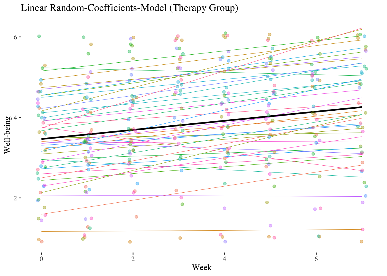
10.4.2 Level-2 models (now including both groups)
In addition to the therapy group \((n = 41)\) the study also included a control group \((n = 44)\). The dummy variable condition is now a level-2 (person) characteristic \(Z\). We expect that the linear increase in well-being is stronger in the therapy group than in the control group (reference category of condition).
10.4.2.1 Slope-as-Outcome Model (Model 5)
Is the cross-level interaction in the expected direction and is it significant?
Let’s estimate a slope-as-outcome model (model with cross-level interaction, model 5) for the entire sample using the level-2 predictor condition.
level-1 model: \(\boldsymbol {WB_{mi}=\beta_{0i} + \beta_{1i} \cdot WEEK_{mi} + \epsilon_{mi}}\)
level-2 model:
\(\boldsymbol {\beta_{0i}=\gamma_{00} + \gamma_{01} \cdot CONDITION_i + \upsilon_{0i}}\)
\(\boldsymbol {\beta_{1i}=\gamma_{10} + \gamma_{11} \cdot CONDITION_i + \upsilon_{1i}}\)
Overall model:
\(\boldsymbol {WB_{mi}=\gamma_{00} + \gamma_{10} \cdot WEEK_{mi} + \gamma_{01} \cdot CONDITION_i + \gamma_{11} \cdot WEEK_{mi} \cdot CONDITION_i +}\) \(\boldsymbol {+ \upsilon_{0i} + \upsilon_{1i} \cdot WEEK_{mi} + \epsilon_{mi}}\)
\(~\)
Important: Now the complete therapy data set has to be used!
slope.outcome <- lme(wellbeing ~ week*condition,
                     random  = ~week | id,
                     data = therapy, method = "ML")
summary(slope.outcome)
## Linear mixed-effects model fit by maximum likelihood
## Data: therapy
## AIC BIC logLik
## 1562.275 1596.941 -773.1373
##
## Random effects:
## Formula: ~week | id
## Structure: General positive-definite, Log-Cholesky parametrization
## StdDev Corr
## (Intercept) 1.0847725 (Intr)
## week 0.1388061 -0.26
## Residual 0.7409710
##
## Fixed effects: wellbeing ~ week * condition
## Value Std.Error DF t-value p-value
## (Intercept) 3.591048 0.18137153 476 19.799404 0.0000
## week -0.007404 0.03038093 476 -0.243695 0.8076
## conditionTherapy -0.133607 0.26096311 83 -0.511975 0.6100
## week:conditionTherapy 0.121185 0.04251483 476 2.850423 0.0046
## Correlation:
## (Intr) week cndtnT
## week -0.393
## conditionTherapy -0.695 0.273
## week:conditionTherapy 0.281 -0.715 -0.400
##
## Standardized Within-Group Residuals:
## Min Q1 Med Q3 Max
## -3.17091725 -0.47081097 0.03428825 0.49678310 3.62043765
##
## Number of Observations: 563
## Number of Groups: 85VarCorr(slope.outcome)## id = pdLogChol(week)
## Variance StdDev Corr
## (Intercept) 1.17673139 1.0847725 (Intr)
## week 0.01926715 0.1388061 -0.26
## Residual 0.54903807 0.7409710The cross-level interaction is positively significant with \(\hat\gamma_{11} = 0.1212\). In the therapy group, the slope of week, i.e. the linear increase in well-being per week, is about 0.12 higher than in the control group.
The main effect of week \((\hat\gamma_{10} = -0.0074)\) is now the conditional effect (simple slope) of week in the control group. Thus, in the control group there is no significant increase in well-being over the course of the seven weeks.
The main effect of condition \((\hat\gamma_{01} = -0.1336)\) is now the difference in well-being between the two groups at the first measurement \((week = 0)\) (baseline).
The difference in well-being at the beginning was therefore not significant.
What proportion of variance of the linear trend of week is explained by condition? We need an additional intercept-as-outcome model (model 4) to answer this.
Intercept-as-outcome model (Model 4)
intercept.outcome <- lme(wellbeing ~ week + condition,
                         random  = ~week | id,
                         data = therapy, method = "ML")
summary(intercept.outcome)
## Linear mixed-effects model fit by maximum likelihood
## Data: therapy
## AIC BIC logLik
## 1567.995 1598.328 -776.9973
##
## Random effects:
## Formula: ~week | id
## Structure: General positive-definite, Log-Cholesky parametrization
## StdDev Corr
## (Intercept) 1.0978853 (Intr)
## week 0.1528630 -0.296
## Residual 0.7401161
##
## Fixed effects: wellbeing ~ week + condition
## Value Std.Error DF t-value p-value
## (Intercept) 3.445564 0.1749101 477 19.699059 0.0000
## week 0.054394 0.0224303 477 2.425020 0.0157
## conditionTherapy 0.165298 0.2391336 83 0.691236 0.4913
## Correlation:
## (Intr) week
## week -0.302
## conditionTherapy -0.659 -0.020
##
## Standardized Within-Group Residuals:
## Min Q1 Med Q3 Max
## -3.126105521 -0.466024855 0.007887938 0.492033076 3.585482735
##
## Number of Observations: 563
## Number of Groups: 85VarCorr(intercept.outcome)## id = pdLogChol(week)
## Variance StdDev Corr
## (Intercept) 1.20535219 1.0978853 (Intr)
## week 0.02336709 0.1528630 -0.296
## Residual 0.54777186 0.7401161Proportion of slope variance explained by condition:
\(R^2_{Cross-level} = \frac{\hat\sigma^2_{\upsilon_14} - \hat\sigma^2_{\upsilon_15}}{\hat\sigma^2_{\upsilon_14}} = \frac{{0.0234} - {0.0193}}{0.0234} = {0.1752}\)
\(\Rightarrow\) 17.52 % of the linear trend variance can be explained by considering the experimental group membership (therapy group versus control group).
Finally, we can check whether the slope variance \({\hat\sigma^2_{\upsilon_1}} = 0.0193\) remaining in Model 5 is still significant. The corresponding model comparison can be obtained via ranova(). This function is only available for models fitted with lmer() from lme4. For the linear trend models it actually makes no difference which of the two functions/packages we use. Therefore we fit model 5 again with lmer().
slope.outcome2 <- lmer(wellbeing ~ week*condition + (week | id),
                       data = therapy, REML = FALSE)
ranova(slope.outcome2)
## ANOVA-like table for random-effects: Single term deletions
##
## Model:
## wellbeing ~ week + condition + (week | id) + week:condition
## npar logLik AIC LRT Df Pr(>Chisq)
## <none> 8 -773.14 1562.3
## week in (week | id) 6 -785.45 1582.9 24.619 2 4.509e-06 ***
## ---
## Signif. codes: 0 '***' 0.001 '**' 0.01 '*' 0.05 '.' 0.1 ' ' 1The comparison shows that a significant interpersonal variance of the linear trend remains even after taking group membership into account. We will not calculate the exact p-value for this comparison at this point.
## `geom_smooth()` using formula 'y ~ x'
## `geom_smooth()` using formula 'y ~ x'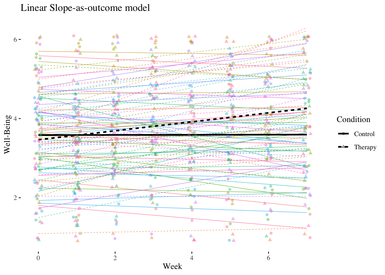
\(~\)
Slope-as-Outcome Model with jamovi/gamlj
GAMLj provides also model diagnostic plots!
gamlj::gamljMixed(
    formula = wellbeing ~ 1 + week + condition + condition:week+( 1 + week | id ),
    data = therapy,
    simpleVariable = week,
    simpleModerator = condition,
    reml = FALSE,
    lrtRandomEffects = TRUE,
    qq = TRUE,
    residPlot = TRUE,
    clusterBoxplot = TRUE,
    randHist = TRUE)
##
## MIXED MODEL
##
## Model Info
## ────────────────────────────────────────────────────────────────────────────────────────────────
## Info
## ────────────────────────────────────────────────────────────────────────────────────────────────
## Estimate Linear mixed model fit by ML
## Call wellbeing ~ 1 + week + condition + condition:week+( 1 + week | id )
## AIC 1562.27450000
## BIC 1596.94070000
## LogLikel. -773.13725309
## R-squared Marginal 0.02852695
## R-squared Conditional 0.69984061
## Converged yes
## Optimizer bobyqa
## ────────────────────────────────────────────────────────────────────────────────────────────────
##
##
## MODEL RESULTS
##
## Fixed Effect Omnibus tests
## ─────────────────────────────────────────────────────────────────
## F Num df Den df p
## ─────────────────────────────────────────────────────────────────
## week 6.305496 1 72.87593 0.0142539
## condition 1.178715 1 86.66718 0.2806284
## week:condition 8.183101 1 72.87593 0.0055134
## ─────────────────────────────────────────────────────────────────
## Note. Satterthwaite method for degrees of freedom
##
##
## Fixed Effects Parameter Estimates
## ─────────────────────────────────────────────────────────────────────────────────────────────────────────────────────────────────────────────
## Names Effect Estimate SE Lower Upper df t p
## ─────────────────────────────────────────────────────────────────────────────────────────────────────────────────────────────────────────────
## (Intercept) (Intercept) 3.69760472 0.12037342 3.46167716 3.93353228 86.66718 30.717785 < .0000001
## week week 0.05318890 0.02118173 0.01167348 0.09470433 72.87593 2.511075 0.0142539
## condition1 Therapy - Control 0.26137558 0.24074683 -0.21047955 0.73323070 86.66718 1.085686 0.2806284
## week:condition1 week:Therapy - Control 0.12118541 0.04236346 0.03815456 0.20421627 72.87593 2.860612 0.0055134
## ─────────────────────────────────────────────────────────────────────────────────────────────────────────────────────────────────────────────
##
##
## Random Components
## ───────────────────────────────────────────────────────────────────
## Groups Name SD Variance ICC
## ───────────────────────────────────────────────────────────────────
## id (Intercept) 1.0613335 1.12642890 0.6723075
## week 0.1388056 0.01926700
## Residual 0.7409708 0.54903779
## ───────────────────────────────────────────────────────────────────
## Note. Number of Obs: 563 , groups: id 85
##
##
## Random Parameters correlations
## ─────────────────────────────────────────────────
## Groups Param.1 Param.2 Corr.
## ─────────────────────────────────────────────────
## id (Intercept) week 0.1607687
## ─────────────────────────────────────────────────
##
##
## Random Effect LRT
## ──────────────────────────────────────────────────────────────────────────────────────
## Test N. par AIC LRT df p
## ──────────────────────────────────────────────────────────────────────────────────────
## week in (1 + week | id) 6 1582.893 24.61890 2.000000 0.0000045
## ──────────────────────────────────────────────────────────────────────────────────────
##
##
## SIMPLE EFFECTS
##
## Simple effects of week : Omnibus Tests
## ─────────────────────────────────────────────────────────────────
## condition F Num df Den df p
## ─────────────────────────────────────────────────────────────────
## Control 0.05800000 1.000000 81.15000 0.8105511
## Therapy 14.30600000 1.000000 79.46000 0.0002996
## ─────────────────────────────────────────────────────────────────
##
##
## Simple effects of week : Parameter estimates
## ───────────────────────────────────────────────────────────────────────────────────────────────────────────────
## condition Estimate SE Lower Upper df t p
## ───────────────────────────────────────────────────────────────────────────────────────────────────────────────
## Control -0.007403804 0.03078536 -0.06865535 0.05384775 81.14510 -0.2404976 0.8105511
## Therapy 0.113781611 0.03008282 0.05390866 0.17365456 79.46037 3.7822793 0.0002996
## ───────────────────────────────────────────────────────────────────────────────────────────────────────────────
##
##
## ASSUMPTION CHECKS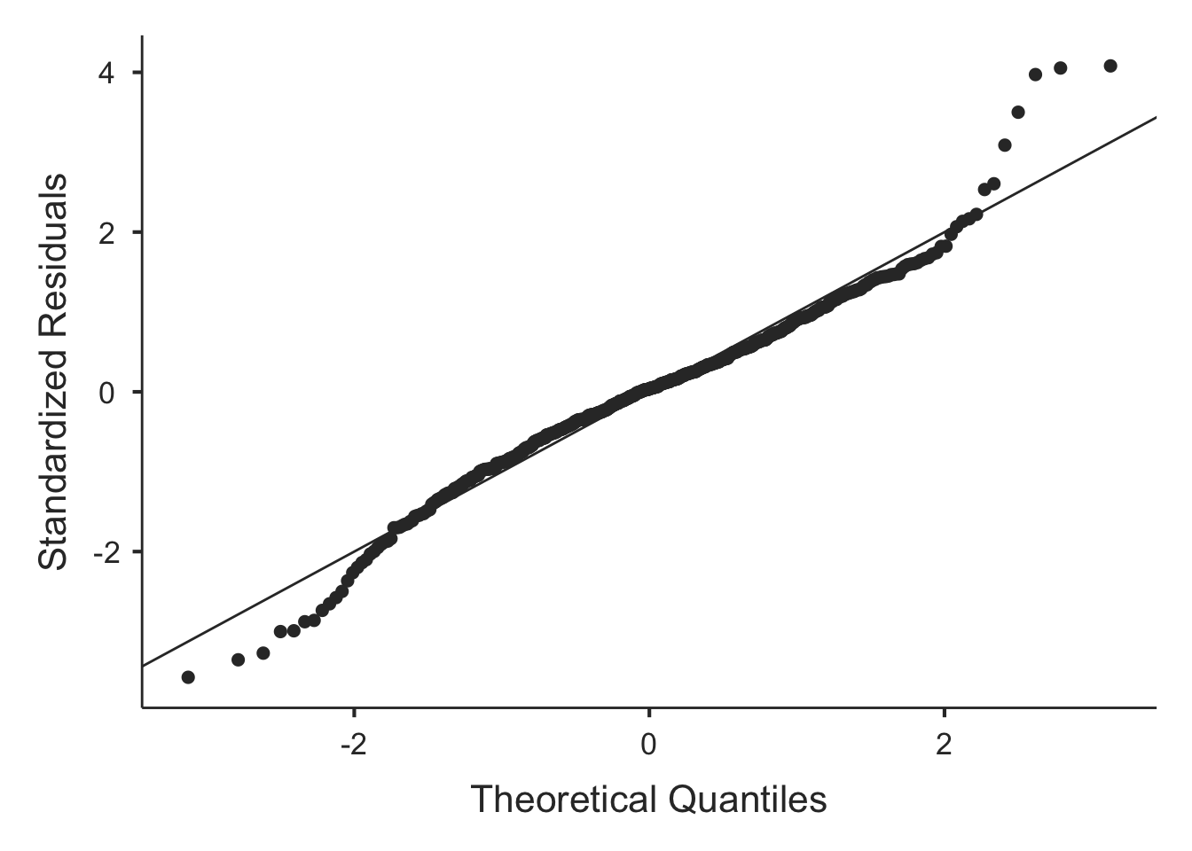
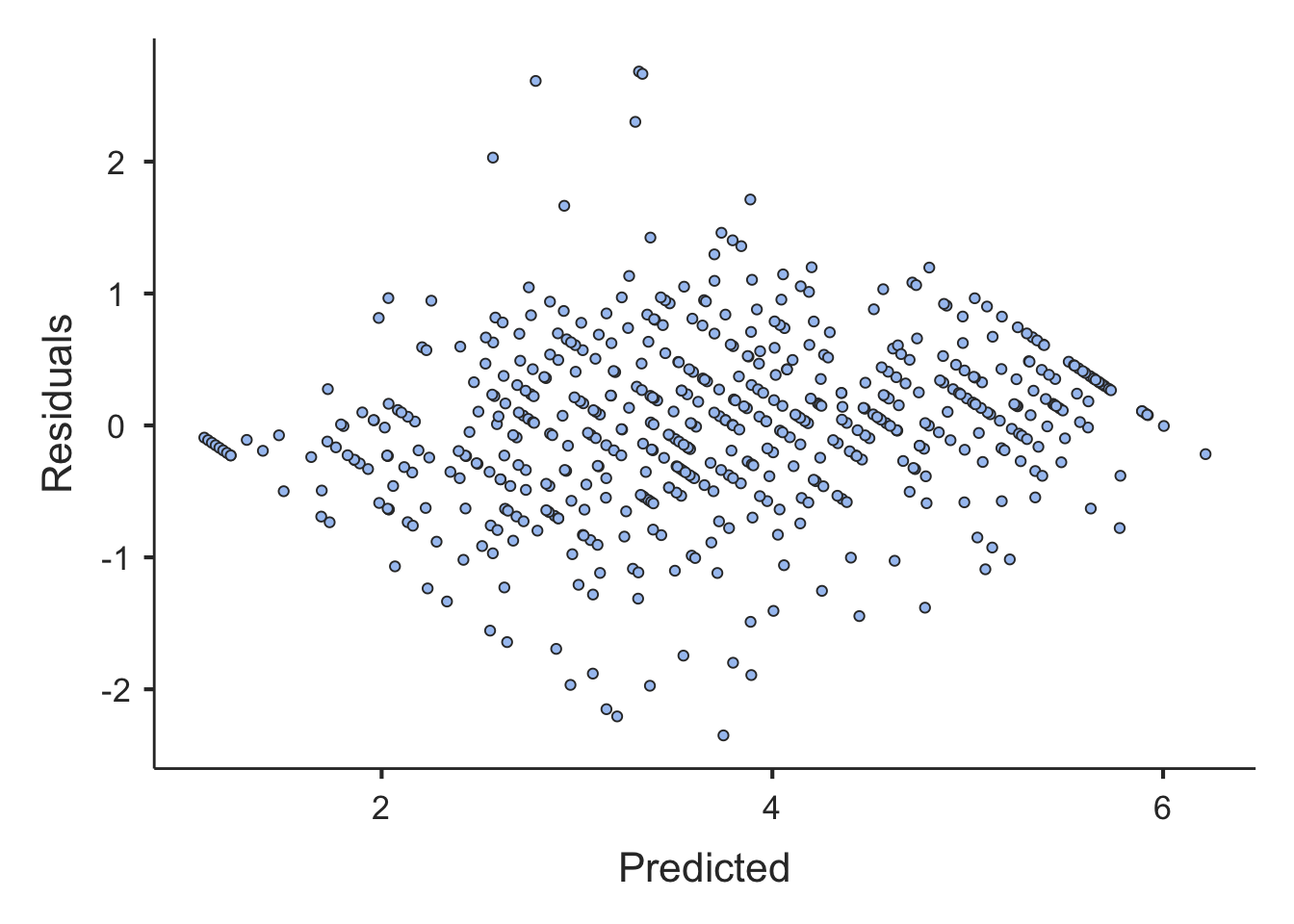
##
  |
  |                                                                      |   0%
  |
  |......................................................................| 100%
##   ordinary text without R code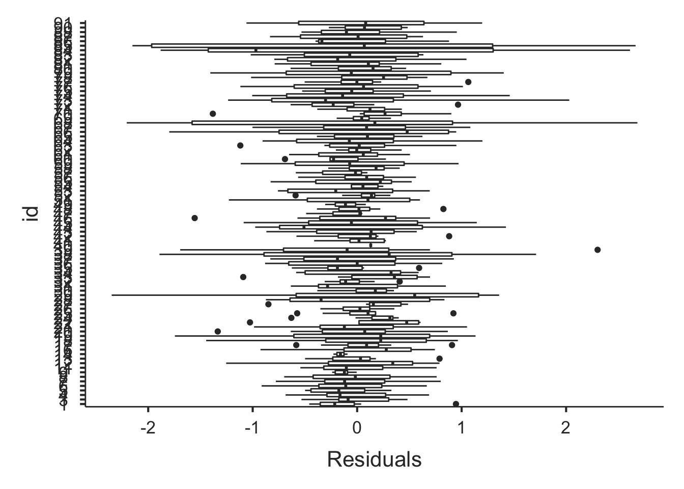
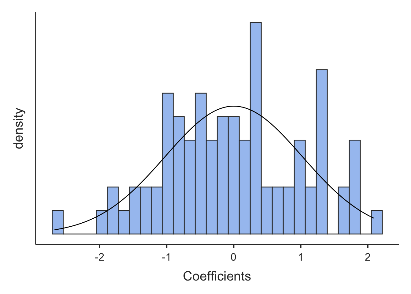
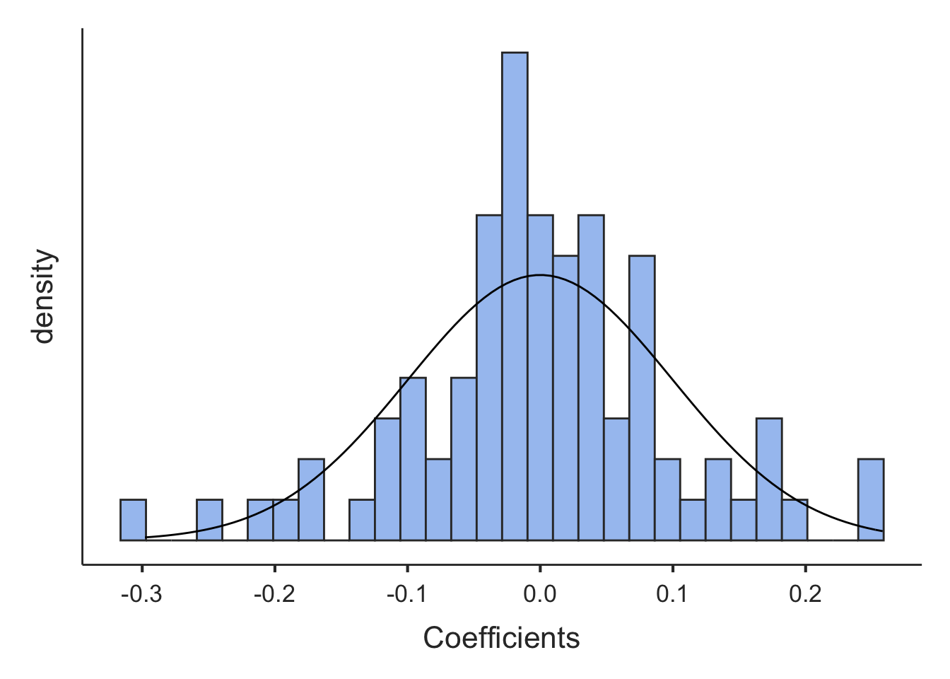
10.4.3 Summary of the linear trend models
In the intercept-only model (model 1) (therapy group only), 57% of the variance of the dependent variable wellbeing was due to differences among individuals.
Even though we have not tested the level-2 variance for significance here, it is obvious that it is substantial and therefore we have to take the person factor into account (a different result would have been very unlikely - there is almost always substantial inter-individual variation in psychological measurements).
In the random intercept model (model 2) (therapy group only) we saw that the effect of week was positively significant, so a constant increase in well-being could be observed in this group. However, this linear trend could only explain about 10% of the within-person (between measurements) variance in well-being. It would be desirable to analyse the differences between the measurement points in more detail using contrast-coded variables (see below).
By comparing the random coefficients Model (model 3) and random intercept model (model 2) we found that the linear increase in well-being differed significantly between individuals, i.e. some individuals showed a stronger and others a weaker (or some even a negative) linear trend in the change of well-being across the treatment period.
In the model with cross-level interaction (model 5), we finally used all data (including the control group) to investigate whether there was a stronger increase in well-being in the therapy group as compared to the control group. The significant and positive CLI showed that this was the case. A substantial percentage (17.5%) of the differences in the linear progress between the individuals was due to group membership. We obtained this value by comparing the slope variances of models 4 and 5.
10.5 Repeated measures HLM: Contrast effect models
We are looking at a contrast model with 6 measuring points (weeks 0-5). The model with all 8 measuring points would need too much computing time due to its complexity.
Let’s get first a data set for the therapy group only that is limited to weeks 0-5 and including the new factor variable week_f:
therapie05_gr1 <- therapy_gr1 %>%
  filter(week <= 5) %>%
  mutate(week_f = as.factor(week))
Also, we need a data set with both groups limited to weeks 0-5:
therapie05 <- therapy %>%
  filter(week <= 5) %>%
  mutate(week_f = as.factor(week))
We also define a special optimizer for ML estimation in lme() to improve the estimation algorithm for these complex models:
opt <- lmeControl(opt = "optim")10.5.1 Level-1 models (therapy group only)
10.5.1.1 Random-Intercept-Model (Model 2)
random.intercept.05.c <- lme(wellbeing ~ week_f,
                             random = ~1 | id,
                             data = therapie05_gr1,
                             method = "ML", control = opt)
summary(random.intercept.05.c)
## Linear mixed-effects model fit by maximum likelihood
## Data: therapie05_gr1
## AIC BIC logLik
## 667.7816 695.1459 -325.8908
##
## Random effects:
## Formula: ~1 | id
## (Intercept) Residual
## StdDev: 1.019026 0.8380026
##
## Fixed effects: wellbeing ~ week_f
## Value Std.Error DF t-value p-value
## (Intercept) 3.298903 0.2127571 180 15.505486 0.0000
## week_f1 -0.029438 0.1933249 180 -0.152271 0.8791
## week_f2 0.593702 0.1975901 180 3.004716 0.0030
## week_f3 0.987673 0.1998182 180 4.942858 0.0000
## week_f4 0.661877 0.1981677 180 3.339985 0.0010
## week_f5 0.713265 0.1965381 180 3.629141 0.0004
## Correlation:
## (Intr) wek_f1 wek_f2 wek_f3 wek_f4
## week_f1 -0.468
## week_f2 -0.456 0.502
## week_f3 -0.454 0.499 0.490
## week_f4 -0.458 0.503 0.494 0.495
## week_f5 -0.461 0.507 0.498 0.496 0.500
##
## Standardized Within-Group Residuals:
## Min Q1 Med Q3 Max
## -2.9664460 -0.5429799 0.0495716 0.5300750 3.0814765
##
## Number of Observations: 226
## Number of Groups: 41VarCorr(random.intercept.05.c)## id = pdLogChol(1)
## Variance StdDev
## (Intercept) 1.0384138 1.0190259
## Residual 0.7022484 0.8380026The results show a non-significant effect of the first dummy variable \((D_1)\) of \(\hat\gamma_{10}= -0.0294\). Between the baseline and week 1 there is therefore no statistically significant change in well-being in the therapy group. In contrast, the effects of the second to fifth dummy variables \((D_2 - D_5)\) are significant with \(\hat\gamma_{20}= 0.5937, \hat\gamma_{30}= 0.9877\), \(\hat\gamma_{40}= 0.6619\), \(\hat\gamma_{50}= 0.7133\). From week 0 to weeks 2, 3, 4 and 5, therefore, a significant increase in well-being is observed.
Is there also a significant overall effect? To evaluate this we have to compare the random intercept model to a model without predictors, i.e. an intercept-only model:
intercept.only.05 <- lme(wellbeing ~ 1,
                         random = ~1 | id,
                         data = therapie05_gr1,
                         method = "ML", control = opt)

anova(random.intercept.05.c, intercept.only.05)
## Model df AIC BIC logLik Test L.Ratio
## random.intercept.05.c 1 8 667.7816 695.1459 -325.8908
## intercept.only.05 2 3 697.8729 708.1345 -345.9365 1 vs 2 40.09131
## p-value
## random.intercept.05.c
## intercept.only.05 <.0001Yes, we can confirm there is also an overall effect/there are overall differences between the 6 measurement points in the variable wellbeing.
10.5.1.2 Random-Coefficients-Model (Model 3)
Now we calculate the random coefficients model including the level-2 variances (and covariances) of the dummy coded time effects.
random.coefficients.05.c <- lme(wellbeing ~ week_f,
                                random = ~week_f | id,
                                data = therapie05_gr1,
                                method = "ML", control = opt)
summary(random.coefficients.05.c)
## Linear mixed-effects model fit by maximum likelihood
## Data: therapie05_gr1
## AIC BIC logLik
## 651.8554 747.6304 -297.9277
##
## Random effects:
## Formula: ~week_f | id
## Structure: General positive-definite, Log-Cholesky parametrization
## StdDev Corr
## (Intercept) 1.2451039 (Intr) wek_f1 wek_f2 wek_f3 wek_f4
## week_f1 0.7981943 -0.251
## week_f2 0.7320714 -0.349 0.130
## week_f3 1.1421484 -0.455 0.192 0.625
## week_f4 1.3916584 -0.500 0.430 0.414 0.608
## week_f5 1.2879439 -0.465 0.104 0.283 0.662 0.898
## Residual 0.3133909
##
## Fixed effects: wellbeing ~ week_f
## Value Std.Error DF t-value p-value
## (Intercept) 3.337590 0.2051562 180 16.268527 0.0000
## week_f1 -0.059225 0.1484191 180 -0.399038 0.6903
## week_f2 0.618723 0.1420465 180 4.355779 0.0000
## week_f3 0.921658 0.2020812 180 4.560829 0.0000
## week_f4 0.589839 0.2361515 180 2.497716 0.0134
## week_f5 0.694226 0.2205398 180 3.147848 0.0019
## Correlation:
## (Intr) wek_f1 wek_f2 wek_f3 wek_f4
## week_f1 -0.313
## week_f2 -0.379 0.237
## week_f3 -0.469 0.255 0.570
## week_f4 -0.514 0.433 0.409 0.582
## week_f5 -0.485 0.182 0.316 0.630 0.851
##
## Standardized Within-Group Residuals:
## Min Q1 Med Q3 Max
## -1.49155839 -0.32707793 0.01418824 0.29089177 1.42247773
##
## Number of Observations: 226
## Number of Groups: 41VarCorr(random.coefficients.05.c)## id = pdLogChol(week_f)
## Variance StdDev Corr
## (Intercept) 1.55028370 1.2451039 (Intr) wek_f1 wek_f2 wek_f3 wek_f4
## week_f1 0.63711410 0.7981943 -0.251
## week_f2 0.53592848 0.7320714 -0.349 0.130
## week_f3 1.30450308 1.1421484 -0.455 0.192 0.625
## week_f4 1.93671311 1.3916584 -0.500 0.430 0.414 0.608
## week_f5 1.65879944 1.2879439 -0.465 0.104 0.283 0.662 0.898
## Residual 0.09821383 0.3133909When we compare this model to the random intercept model, we get a significance test for the variances and covariances of the effects of dummy variables (dummy-coded effects) 1-5. We naturally assume that such variances and covariances do exist since there is no reason to assume that the well-being of all patients would change in exactly the same way over the six measurement points and also that the effects would be uncorrelated.
anova(random.coefficients.05.c, random.intercept.05.c)## Model df AIC BIC logLik Test L.Ratio
## random.coefficients.05.c 1 28 651.8554 747.6304 -297.9277
## random.intercept.05.c 2 8 667.7816 695.1459 -325.8908 1 vs 2 55.92619
## p-value
## random.coefficients.05.c
## random.intercept.05.c <.0001The random coefficients model estimates 28 parameters while the random intercept model estimates only 8 parameters. The difference in the deviances is \((-2\cdot logLik_{RI})- (-2\cdot logLik_{RC})= [-2\cdot (-325.8908)] - [-2\cdot (-297.9277)] =\) \(651.7816 - 595.8554 = 55.9262\), and this is approximately \(\chi^2\)-distributed with \(df=npar_{RC}-npar_{RI} = 28-8 = 20\) and with a \(p<.0001\). Again, one could determine an even more precise p-value of a complex mixture distribution, but this would be very laborious because of the large number of parameters involved (as well as unnecessary in light of the very low obtained p-value).
Overall, the variances and covariances of the dummy effects are therefore statistically significant.
10.5.1.3 Compare to the linear model
It could be that the linear RC model calculated above is sufficient to model the change in well-being over time. We can check this by comparing the RC contrast model with the linear RC model. We have calculated the linear model above for all measurement points (0-7). Therefore we have to calculate it again restricted to the first six measurement points in order to be able to carry out the comparison.
random.coefficients.05.l <- lme(wellbeing ~ week,
                                random = ~week | id,
                                data = therapie05_gr1,
                                method = "ML", control = opt)

anova(random.coefficients.05.c, random.coefficients.05.l)
## Model df AIC BIC logLik Test L.Ratio
## random.coefficients.05.c 1 28 651.8554 747.6304 -297.9277
## random.coefficients.05.l 2 6 664.6327 685.1560 -326.3164 1 vs 2 56.77733
## p-value
## random.coefficients.05.c
## random.coefficients.05.l 1e-04The linear model fits the data significantly worse than the contrast model. Therefore, it is necessary to consider the non-linear parts of the curve.
One could now also check whether a polynomial trend model (with a quadratic, cubic or quartic effect) is sufficient, i.e. whether the non-linearity of the trend does not necessarily have to be described by the highest-order contrast model. It might be possible to stay with a (somewhat) more parsimonious model. However, this is not the case (with regard to the random coefficients model). We do not report the results of these model comparisons here due to the extensive computing time these models require.
\(~\)
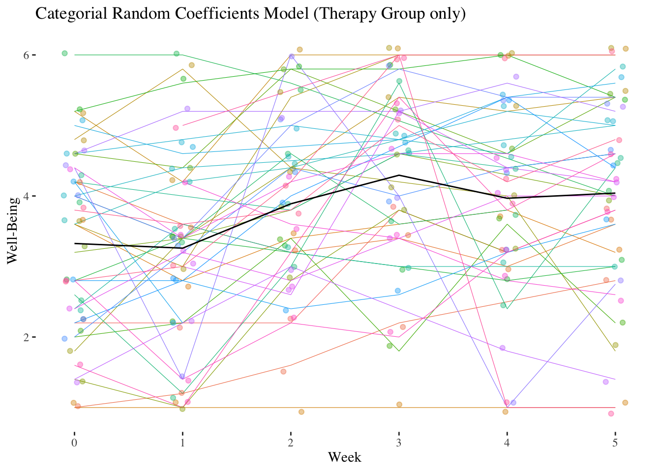 \(~\)
\(~\)
\(~\)
\(~\)
\(~\)
\(~\)
## `geom_smooth()` using formula 'y ~ x'
## `geom_smooth()` using formula 'y ~ x'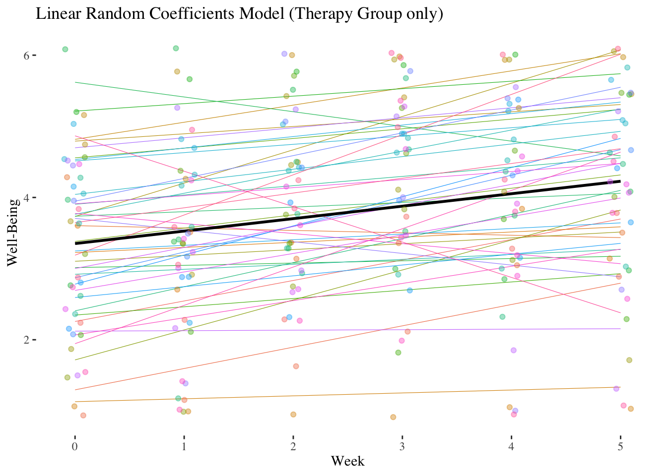
10.5.2 Level-2 models (therapy and control group)
10.5.2.1 Slope-as-Outcome Model (Model 5)
We start right away with the slope-as-outcome model, because this model contains everything we are interested in when we analyze both groups (therapy and control group).
The cross-level interaction contained in this model tests the difference in dummy variable effects between the therapy and control groups. A positive CLI means that the corresponding effect is stronger in the therapy group than in the control group.
This model has to be estimated using the complete data set (all groups) for weeks 0-5:
slope.outcome.05.c <- lme(wellbeing ~ week_f*condition,
                          random = ~week_f | id,
                          data = therapie05,
                          method = "ML", control = opt)
summary(slope.outcome.05.c)
## Linear mixed-effects model fit by maximum likelihood
## Data: therapie05
## AIC BIC logLik
## 1240.495 1379.523 -586.2475
##
## Random effects:
## Formula: ~week_f | id
## Structure: General positive-definite, Log-Cholesky parametrization
## StdDev Corr
## (Intercept) 1.3032731 (Intr) wek_f1 wek_f2 wek_f3 wek_f4
## week_f1 0.8383595 -0.380
## week_f2 0.7418214 -0.422 0.377
## week_f3 0.9517854 -0.430 0.291 0.569
## week_f4 1.3432213 -0.542 0.725 0.594 0.658
## week_f5 1.4010005 -0.543 0.436 0.422 0.714 0.864
## Residual 0.3576422
##
## Fixed effects: wellbeing ~ week_f * condition
## Value Std.Error DF t-value p-value
## (Intercept) 3.829804 0.2073060 346 18.474160 0.0000
## week_f1 -0.479348 0.1521362 346 -3.150782 0.0018
## week_f2 -0.334772 0.1453397 346 -2.303376 0.0219
## week_f3 -0.204482 0.1825410 346 -1.120195 0.2634
## week_f4 -0.290526 0.2345400 346 -1.238707 0.2163
## week_f5 -0.114596 0.2506857 346 -0.457131 0.6479
## conditionTherapy -0.433190 0.2996694 83 -1.445560 0.1521
## week_f1:conditionTherapy 0.357137 0.2203293 346 1.620926 0.1059
## week_f2:conditionTherapy 0.886342 0.2085806 346 4.249397 0.0000
## week_f3:conditionTherapy 1.075384 0.2562673 346 4.196336 0.0000
## week_f4:conditionTherapy 0.821218 0.3301801 346 2.487182 0.0133
## week_f5:conditionTherapy 0.732588 0.3480789 346 2.104660 0.0360
## Correlation:
## (Intr) wek_f1 wek_f2 wek_f3 wek_f4 wek_f5 cndtnT
## week_f1 -0.412
## week_f2 -0.426 0.403
## week_f3 -0.413 0.313 0.481
## week_f4 -0.523 0.635 0.513 0.548
## week_f5 -0.507 0.401 0.373 0.571 0.775
## conditionTherapy -0.692 0.285 0.295 0.286 0.362 0.350
## week_f1:conditionTherapy 0.284 -0.690 -0.278 -0.216 -0.439 -0.277 -0.419
## week_f2:conditionTherapy 0.297 -0.281 -0.697 -0.335 -0.357 -0.260 -0.435
## week_f3:conditionTherapy 0.294 -0.223 -0.343 -0.712 -0.390 -0.407 -0.433
## week_f4:conditionTherapy 0.372 -0.451 -0.364 -0.389 -0.710 -0.550 -0.540
## week_f5:conditionTherapy 0.365 -0.289 -0.269 -0.412 -0.558 -0.720 -0.531
## wk_1:T wk_2:T wk_3:T wk_4:T
## week_f1
## week_f2
## week_f3
## week_f4
## week_f5
## conditionTherapy
## week_f1:conditionTherapy
## week_f2:conditionTherapy 0.411
## week_f3:conditionTherapy 0.333 0.507
## week_f4:conditionTherapy 0.651 0.530 0.580
## week_f5:conditionTherapy 0.423 0.397 0.613 0.792
##
## Standardized Within-Group Residuals:
## Min Q1 Med Q3 Max
## -1.71991243 -0.33295766 0.01480146 0.30317798 1.82739628
##
## Number of Observations: 441
## Number of Groups: 85VarCorr(slope.outcome.05.c)## id = pdLogChol(week_f)
## Variance StdDev Corr
## (Intercept) 1.6985207 1.3032731 (Intr) wek_f1 wek_f2 wek_f3 wek_f4
## week_f1 0.7028467 0.8383595 -0.380
## week_f2 0.5502990 0.7418214 -0.422 0.377
## week_f3 0.9058955 0.9517854 -0.430 0.291 0.569
## week_f4 1.8042436 1.3432213 -0.542 0.725 0.594 0.658
## week_f5 1.9628023 1.4010005 -0.543 0.436 0.422 0.714 0.864
## Residual 0.1279079 0.3576422The results show that all but the first of the interaction terms are significant. Only from week 0 to week 1 (interaction term \(D_1 \times Z: \hat\gamma_{11}= 0.3571\)) the difference between therapy and control group is not significant. For all other contrasts with the baseline there is a significant difference in the change in well-being: Week 2 (interaction term \(D_2 \times Z: \hat\gamma_{21}= 0.8863\)), week 3 (interaction term \(D_3 \times Z: \hat\gamma_{31}= 1.0754\)), week 4 (interaction term \(D_4 \times Z: \hat\gamma_{41}= 0.8212\)), week 5 (interaction term \(D_5 \times Z: \hat\gamma_{51}= 0.7326\)).
The simple slopes of week_fare also interesting (i.e. the effects of the dummy variables \(D_1 - D_5\)): These conditional effects test the changes within the control group (reference category of condition). In this group well-being is significantly reduced across the first two weeks before it stabilizes (no significant contrasts with the baseline are observed from week 3).
Strictly speaking, we still need a test for the overall effect of the interaction (i.e. all five interaction terms together). We get this by comparing it with a model that does not contain a CLI:
intercept.outcome.05.c <- lme(wellbeing ~ week_f + condition,
                              random = ~week_f | id,
                              data = therapie05,
                              method = "ML", control = opt)

anova(slope.outcome.05.c, intercept.outcome.05.c)
## Model df AIC BIC logLik Test L.Ratio
## slope.outcome.05.c 1 34 1240.495 1379.523 -586.2475
## intercept.outcome.05.c 2 29 1251.700 1370.283 -596.8503 1 vs 2 21.20549
## p-value
## slope.outcome.05.c
## intercept.outcome.05.c 7e-04The overall cross-level interaction is thus also significant!
10.5.2.2 Comparison with the linear model
Again, a linear model may be sufficient to model the change in well-being over time. Again, we can test this by comparing the slope-as-outcome contrast model to a slope-as-outcome linear model:
slope.outcome.05.l <- lme(wellbeing ~ week*condition, random = ~week | id,
                           data = therapie05, method = "ML", control = opt)

anova(slope.outcome.05.c, slope.outcome.05.l)
## Model df AIC BIC logLik Test L.Ratio p-value
## slope.outcome.05.c 1 34 1240.495 1379.523 -586.2475
## slope.outcome.05.l 2 8 1261.812 1294.524 -622.9058 1 vs 2 73.31663 <.0001Here, too, the LR test shows that the contrast model is clearly to be preferred over the linear model.
\(~\)
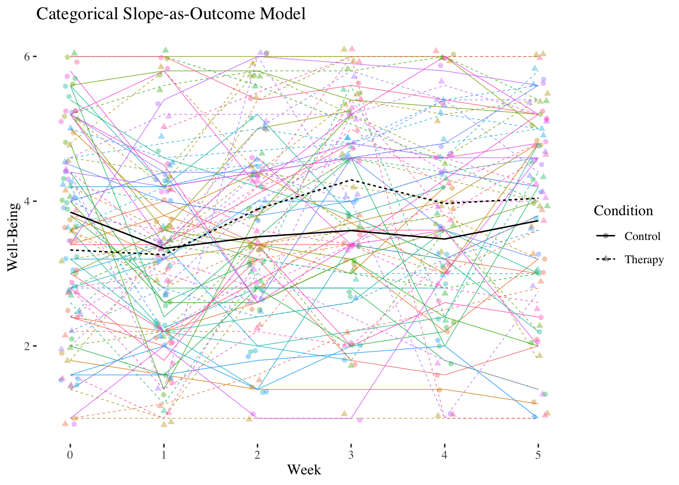
\(~\) \(~\) \(~\)
## `geom_smooth()` using formula 'y ~ x'
## `geom_smooth()` using formula 'y ~ x'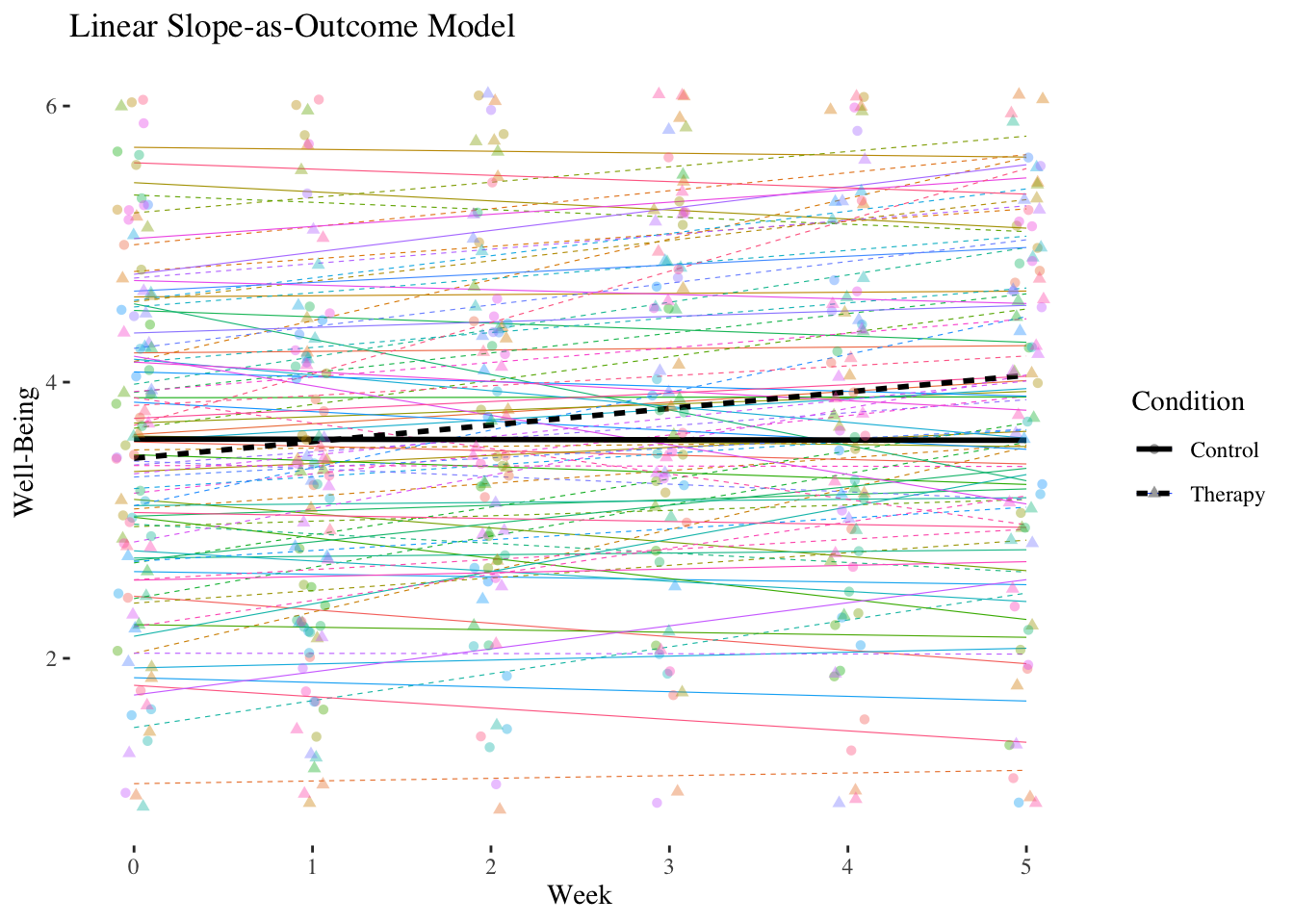
10.5.3 Summary of the contrast effect models
The RI-contrast model (model 2) (therapy group only) showed significant increases in well-being over the five weeks of therapy. Only the well-being measured after the first week was not significantly higher than baseline well-being, all other contrasts to baseline were significant. Because of the dummy coding we can only make statements about the baseline contrasts. Using this kind of contrast coding we cannot determine whether the well-being also improved significantly between the individual weeks (e.g. from week 2 to week 3). To test this, we would need to employ repeated contrasts coding. Furthermore, a model comparison with an intercept-only model (model 1) showed that the overall effect of the week factor was significant, and thus total differences in well-being over time were confirmed.
The RC-contrast model (model 3) estimated the variances and covariances of these effects in addition to the average (=fixed) effects of the week factor. These were not discussed in detail above, partly because they are usually not the focus of the research. On the one hand, it appeared that the variances of the weekly effects tended to increase with the distance from the baseline, i.e. that the interindividual differences in the well-being change (i.e. compared to the well-being at the beginning) became larger in the course of the therapy. Furthermore, negative correlations of the person-specific intercept with the effects of weeks 1-5 were observed: Participants who had already started with a higher level of well-being tended to show a lower improvement in well-being than those with a lower level of well-being at the beginning. In contrast, the effects of weeks 1-5 were all positively correlated: Persons who showed a stronger change in well-being e.g. from the baseline to week 2also showed a stronger change from the baseline to week 3 (\(r_{\upsilon_2 \upsilon_3}=0.625\)). The model comparison of the RC model to the RI model showed that these variances and covariances can be considered statistically significant overall. In addition, by comparing the RC model with a linear RC model, we checked whether the linearity assumption we had made in the first part of this exercise was appropriate. Since the linear model fitted the data significantly worse than the contrast model, the latter is to be preferred. The changes over the course of therapy are therefore not linear, but there are “jumps and bumps”. In particular, the improvement in well-being appears to be strongest between weeks 1 and 3.
However, the main focus of these analyses was on the Slope-as-Outcome Contrast Model (Model 5)), which was calculated using the complete data set (therapy and control group). Here, as in the linear slope-as-outcome model, significant differences between therapy and control group were found with regard to the change in well-being over the course of therapy: With the exception of the change from the baseline to the first week, where no significant difference was found between therapy and control group, all other comparisons with the baseline showed that the change (improvement) in well-being was stronger in the therapy group than in the control group. A comparison of this model to a model without any cross-level interaction term (model 4) showed that the interaction of week and group membership can also in total be considered statistically significant. Finally, it was also checked whether a linear model would be sufficient here. Since the LR test of the model comparison with the corresponding (i.e. limited to weeks 0-5) linear slope-as-outcome model was significant, the null hypothesis that the linear model does not fit worse compared to the contrast model had to be rejected. Thus, a linear trend model is not sufficient to describe the differences in the change of well-being between therapy and control group. The figures illustrate the two different models conclusively.