1 RStudio workflow

1.1 Graphical user interface (GUI)

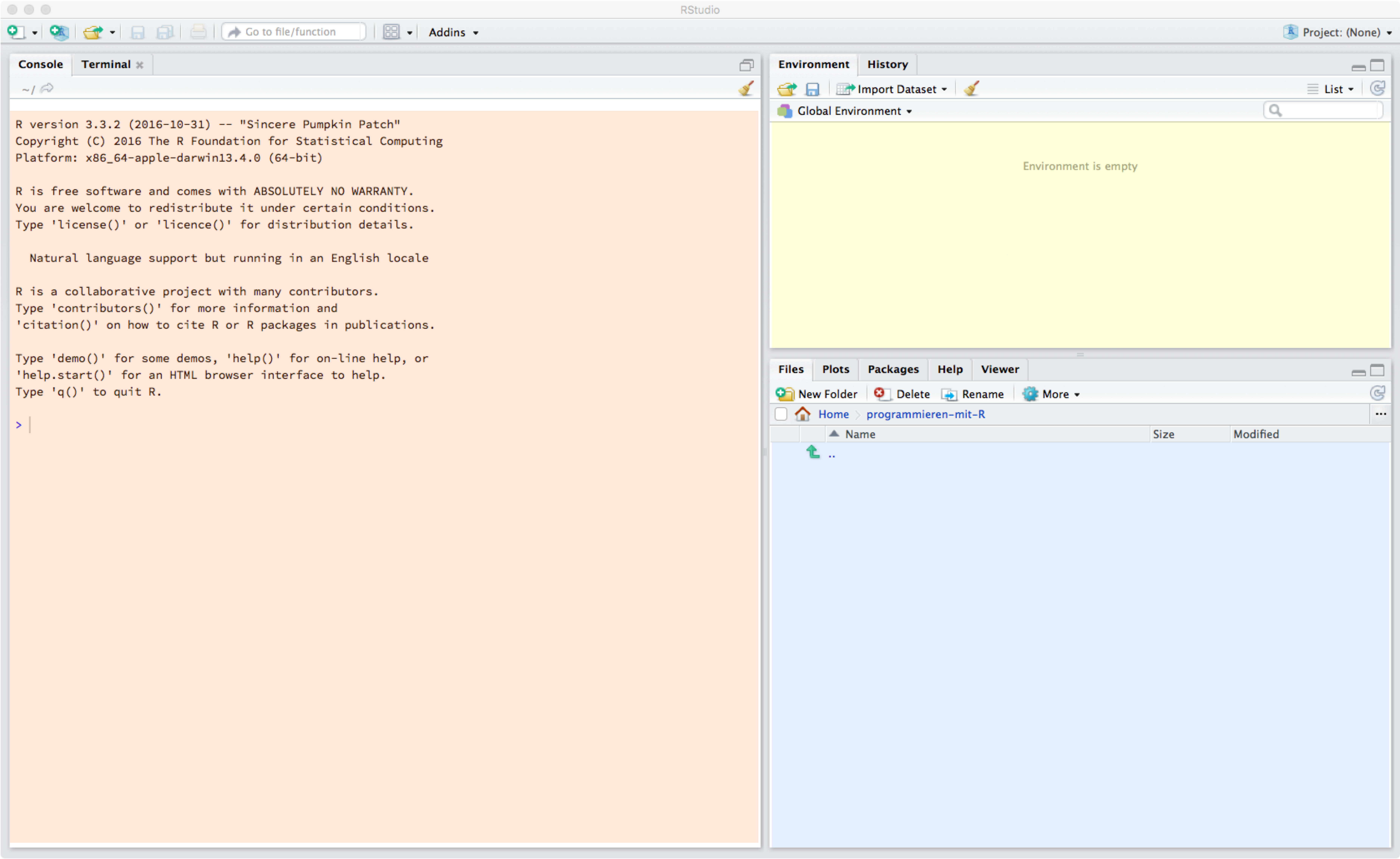
Let’s begin by exploring RStudio. When you open the program, it should look something like this:

1.1.1 Preferences

Under the Preferences or Global Options menu items, you can customize RStudio. We recommend not using the following options:

Restore .RData into workspace at startup (Do not activate this)
Save workspace to .RData on exit (Never) (Do not activate this)

It’s best to start each session with an empty workspace.

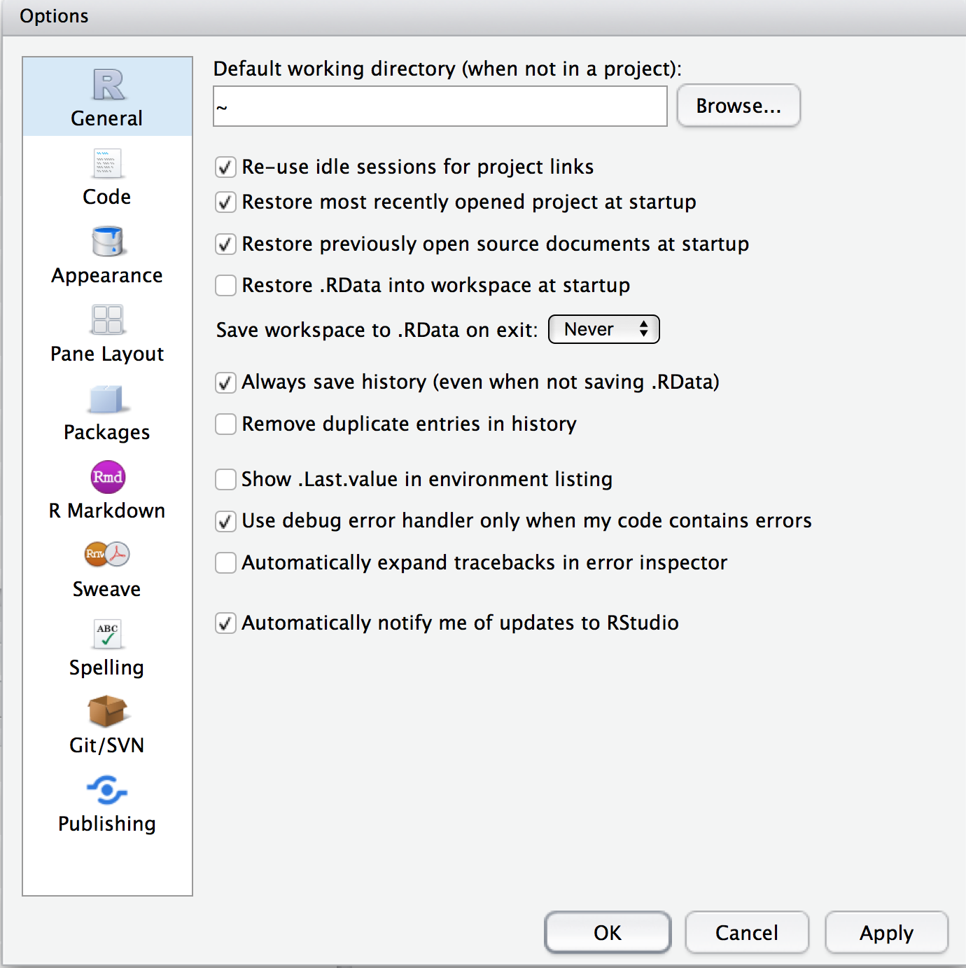
You can change many settings relating to appearance and layout here.

1.1.2 Panes

The RStudio GUI is composed of several panes. On the left is the R console (orange). This is where you can directly interact with R. If you enter a command here, and press Enter, the command will be interpreted by R.

The > symbol is called the R prompt. You can try to use R as a calulator:

2 + 3

## [1] 5

exp(1)

## [1] 2.718282

3/4

## [1] 0.75

Top right (yellow): here, we have two panes Environment and History. In the Environment pane RStudio shows us all variables, datasets and functions that are available in the current session. If you click on the Global Environment drop-down menu, you can see which packages have been loaded.

The History pane shows a history of all commands that we have entered.

Bottom right (blue): here, we have the Files (file manager), Plots, Packages and Help Viewer panes.

Using the file manager, you can switch working directories and open files:

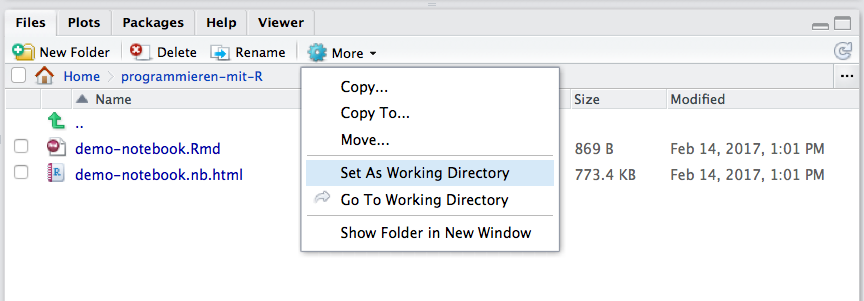
If you change working directories using the file manager, R will display the command in the console. In this case, the R command is setwd(...). By entering getwd(), you can ask R which directory you are currently in.

1.2 Packages

Before we start, we need to install some packages. Packages provide functionality that is not available in base R. We will need packages for importing (readr, readxl, haven) and manipulating data (tidyr, dplyr, forcats, tibble), as well as for plotting (ggplot2).

We can install all of these with the meta-package tidyverse using the command:

install.packages("tidyverse")

You only need to do this once. Installed packages are stored on your computer in a place where R can find them. However, to make them available in an R session, we need to load packages using the library command:

library(tidyverse)

Important note: Though many more packages are installed when installing the meta-package tidyverse, only the most important of these are loaded with library(tidyverse). These core parts of the tidyverse are the (sub-)packages tidyr, dplyr, forcats, readr, ggplot2, tibble (we will use these later) as well as purrr and stringr (which we will not use in this course). Packages that are installed with the tidyverse but need to be loaded separately are, e.g., haven (for importing data from SPSS) and readxl (for importing data from Excel). We will come back to this later.

We can also use the GUI for installing and loading packages:

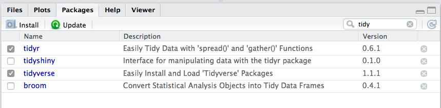
It’s a good idea to keep all packages up to date. You can use (Update) in the Packages pane or, if you prefer:

update.packages(ask = FALSE)

R Packages are hosted on a server: The Comprehensive R Archive Network, or CRAN. Have a look at Task Views; these show a collection of packages for various topics, e.g. psychometrics CRAN Task View: Psychometric Models and Methods.

1.3 Help

In case you get stuck, RStudio has a built-in Help viewer:

You can either enter a search term in the Help Viewer, or you can browse the packages to access their help pages.

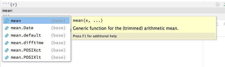
You can also access help directly in the console:

help(mean)

This will open the help page for the mean function. You can also enter ?mean.

A very useful source of information is the Q & A website Stackoverflow - here you will discover you are not the first person to encounter a particular problem, and that someone has most likely already figured out a solution.

1.4 Working with RStudio

1.4.1 Projects

We recommend that you always work in a project. A project specifies your working directory, workspace, history, and source documents.

You can create a new project under the File menu (“File -> New Project…”). You will be asked whether you would like to create the project in a new directory or in an existing directory. The best strategy is to prepare a folder in your file system that you plan to use for all files related to the new project and then use this ‘Existing Directory’. In this script

The created project file end with .Rproj and functions as a container of or gateway to your project: If you start RStudio by double-clicking this file in your file system, RStudio will run “in project mode” meaning that the working directory is automatically set to the folder the project file resides in. This has a number of advantages: e.g., no need to specify working directory, no need to use absolute paths for referring to data files etc.

We also recommend creating a subfolder data in your project folder since we will always use a relative path to example data files that reside in the data subfolder of your project folder in this script.

1.4.2 Console

You can either enter commands directly into the console, or write in a text file, and then send the command to the console.

Working in the console is ok for quickly trying things out, but usually it is better to use text files (see next section).

This ensures that you keep a record of what you did, and in which order you did it. This is very important for ensuring reproducibility, not just for other researchers, but also for your future self.

You can access your latest commands in the console using the Up key (several times for earlier commands). Once you used the Up key (several times) you can use the Down key to access later commands. This is useful when you want to do something again or do something very similar by adjusting earlier commands.

If you forget to complete an R command, you might see this:

> mean(x
+

This means that R is waiting for you to complete the command. In this case, you can either enter ) or press ESCAPE or CTRL-C. With ) you correctly finish the command, with ESCAPE or CTRL-C you get a new prompt and can start over.

1.4.3 R Script

Let’s open an R script (text file with the file ending .R). Enter the R code: 2 + 3

Then you can select the code, and click on Run button. This will evaluate the selected code, and you will see the output in the console. Instead of clicking on the button, you can use the shortcut CTRL-Enter.

Another example: Enter and run the following code in your new R script: x <- c(101, 105, 99, 87, 102, 98)

You just defined a vector (or a variable). Since there is no output when ‘only’ defining somehting you will see only the (copied) entered command in the output (and the prompt > indicating the start of a new line):

> x <- c(101, 105, 99, 87, 102, 98)

But still something happened: in the Environment you will see that x is a num [1:6]. This means that x is a numeric vector with length 6, i.e. consisting of 6 elements.

If you want to see the contents of x, you can type x and evaluate (in this case: print) it. You could also use print(x).

The output in the console will be: [1] 101 105 99 87 102 98

Try also running: boxplot(x) You should see a box plot in the Plots pane in the lower right of RStudio.

1.4.4 Using R Notebooks

R Notebooks are interactive RMarkdown documents (RMarkdown is a simple markup language). These can display text, code and graphics, all in the same document.

Open a new notebook file:

You can save the notebook with the file ending .Rmd.

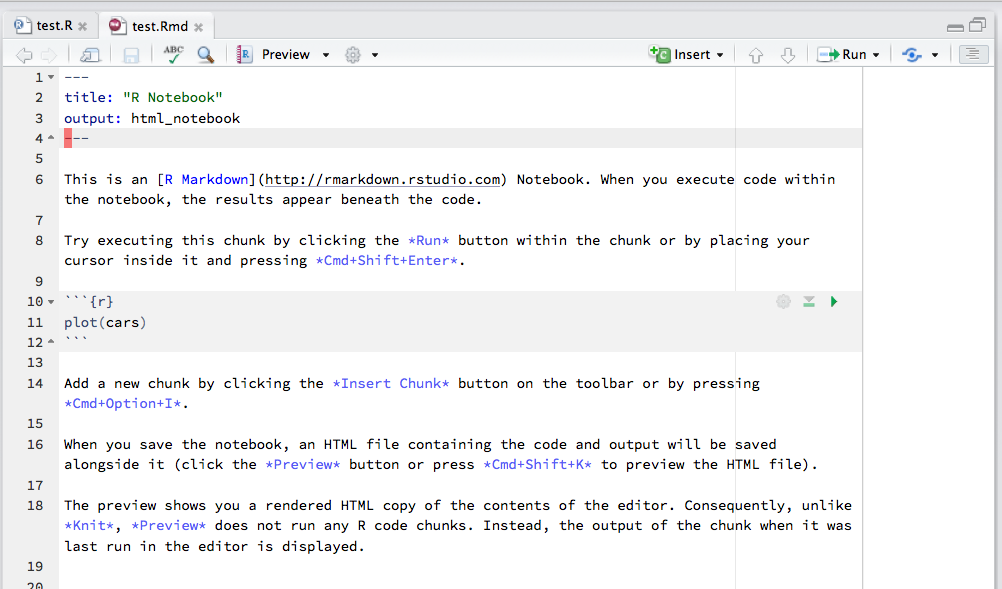
Notebooks contain both Markdown text and code chunks. These code chunks can be evaluated.

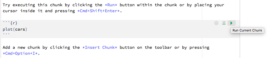
When you press the green arrow the output will appear right beneath the code chunk.

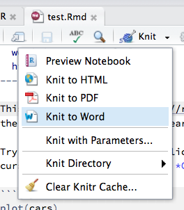
The whole document can be compiled by clicking on Preview. The first time you do this, RStudio will ask you to install some missing packages (you should do this). After compilation, you will see an HTML document in the Viewer pane. You can also create Word documents or PDFs:

1.4.5 Tab completion

RStudio has a very useful feature: tab completion. If you enter R commands in the console or in the text editor, you will automatically be provided you with a list of possible completions. We can also get suggestions, including possible arguments of functions, by pressing the tab key.

We can also use this feature to look for functions inside packages. For example, we can write a package name, followed by :: and the press tab. RStudio will give us a list of functions from that package. To get a list of all functions starting with the letter f from the dplyr package:

dplyr::f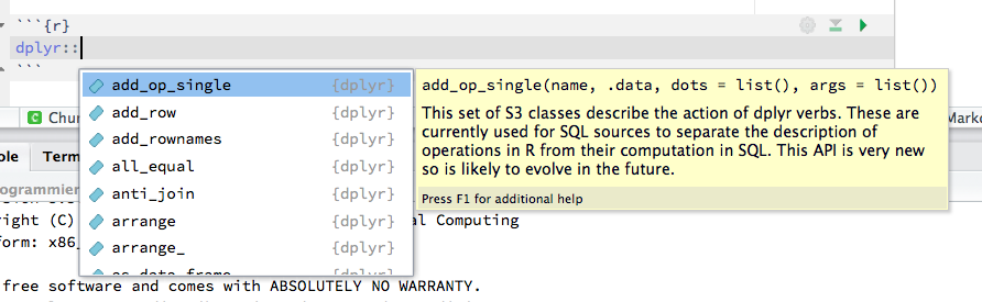

1.4.6 Key combinations

We will need the following symbols:

[ ]  Square braces
{ }  Curly braces
$    Dollar key
#    Hash (pound) key
~    Tilde (for formula notation)
|    Vertical bar
`    Backtick

Unfortunately, these can be somewhat difficult to find on German/Swiss keyboards. Take a few minutes to familiarize yourself with your keyboard. You will need to use the ALT key for some of the symbols.