9 Linear models
9.1 Multiple regression
In a linear (multiple) regression model we are interested in the joint linear prediction of a dependent variable by one or more independent variables. By taking into account the interdependencies among the predictor (independent) variables we aim to assess the unique effect of each predictor in the context of all other predictors.
The regression equation for three predictor variables is:
Population model:
\(Y = \beta_0 + \beta_1 \cdot X_1 + \beta_2 \cdot X_2 + \beta_3 \cdot X_3 + E\)
Sample model:
\(Y = b_0 + b_1 \cdot X_1 + b_2 \cdot X_2 + b_3 \cdot X_3 + E\)
We can also write the regression equation for the predicted values (\(\hat Y\)) by omitting the residual variable \(E\):
\(\hat Y = b_0 + b_1 \cdot X_1 + b_2 \cdot X_2 + b_3 \cdot X_3\)
The regression model above is specified as follows using the lm()function:
lm(Y ~ X1 + X2 + X3, data = mydata).
The formula notation is the same as used earlier with aov() to analyze factorial ANOVAS. Connecting the predictor variables using + means that only main effects will be estimated (multiple regression). If we want a model including all possible (two-way and three-way interactions) the predictors have to be linked using *. If only certain interaction effects should be in the model, the respective predictors are connected using : and the corresponding terms are added using +.
For example, lm(Y ~ X1 + X2 + X3 + X1:X2 + X2:X3 + X1:X3, data = mydata) represents a model with all main effects and all two-way interactions, but without the three-way interaction X1:X2:X3.
Before we start with an example, a new way of loading and installing packages is introduced. The function p_load() from the pacman package allows loading a number of packages and automatically installs packages that cannot be found on the system:
install.packages("pacman")
pacman::p_load(haven, interactions, memisc, QuantPsyc, psych, tidyverse, jtools)As a first example, let us predict adolescents’ overall grade average by the three subscales from the academic self-efficacy domain. The data set should thus include the variables ID and grade_overall, as well as se_achievement, se_learning, and se_motivation (the three academic self-efficacy subscales). Since we will be adding the three subscales from the social self-efficacy domain in a subsequent example the scales se_assertive, se_social, and se_relationships are also included.
Loading and preparing the data set segrade:
load(file = "data/adolescents.Rdata")
segrade <- adolescents %>%
    dplyr::select(ID, grade_overall, starts_with("se")) %>%
    drop_na()
Let’s have a look at the data and get some descriptive statistics plus a bivariate correlation matrix:
head(segrade)## # A tibble: 6 × 8
## ID grade_overall se_achievement se_learning se_motivation se_assertive
## <fct> <dbl> <dbl> <dbl> <dbl> <dbl>
## 1 2 4 5 4 4.6 5
## 2 10 5 5 4.88 6 4.33
## 3 11 4 4.57 5.38 5.4 5.33
## 4 12 5 5.33 5.29 4.67 4.67
## 5 14 4 4.86 4.5 4.6 5.33
## 6 15 4 4 4.38 5.6 4.33
## # … with 2 more variables: se_social <dbl>, se_relationships <dbl>describe(segrade[,-1], fast = TRUE)## vars n mean sd min max range se
## grade_overall 1 279 4.46 0.69 3.00 6 3.00 0.04
## se_achievement 2 279 5.09 0.78 2.43 7 4.57 0.05
## se_learning 3 279 5.23 0.80 2.88 7 4.12 0.05
## se_motivation 4 279 5.44 0.76 3.20 7 3.80 0.05
## se_assertive 5 279 5.28 0.99 1.00 7 6.00 0.06
## se_social 6 279 5.28 0.79 1.57 7 5.43 0.05
## se_relationships 7 279 5.61 0.75 3.33 7 3.67 0.05segrade %>%
dplyr::select(-ID) %>%
cor() %>%
round(2)## grade_overall se_achievement se_learning se_motivation
## grade_overall 1.00 0.42 0.39 0.34
## se_achievement 0.42 1.00 0.56 0.64
## se_learning 0.39 0.56 1.00 0.72
## se_motivation 0.34 0.64 0.72 1.00
## se_assertive 0.05 0.34 0.31 0.42
## se_social 0.11 0.36 0.33 0.41
## se_relationships 0.24 0.39 0.46 0.41
## se_assertive se_social se_relationships
## grade_overall 0.05 0.11 0.24
## se_achievement 0.34 0.36 0.39
## se_learning 0.31 0.33 0.46
## se_motivation 0.42 0.41 0.41
## se_assertive 1.00 0.59 0.32
## se_social 0.59 1.00 0.49
## se_relationships 0.32 0.49 1.00Estimation of the regression model:
model_1 <- lm(grade_overall ~ se_achievement + se_learning + se_motivation,
              data = segrade)
Results with summary(), confidence intervals with confint(), and standardized regression coefficients with QuantPsyc::lm.beta()
summary(model_1)##
## Call:
## lm(formula = grade_overall ~ se_achievement + se_learning + se_motivation,
## data = segrade)
##
## Residuals:
## Min 1Q Median 3Q Max
## -1.63155 -0.42393 0.06732 0.46759 1.27122
##
## Coefficients:
## Estimate Std. Error t value Pr(>|t|)
## (Intercept) 2.13666 0.28957 7.379 1.90e-12 ***
## se_achievement 0.26849 0.06352 4.227 3.23e-05 ***
## se_learning 0.20282 0.06773 2.995 0.003 **
## se_motivation -0.01869 0.07679 -0.243 0.808
## ---
## Signif. codes: 0 '***' 0.001 '**' 0.01 '*' 0.05 '.' 0.1 ' ' 1
##
## Residual standard error: 0.6176 on 275 degrees of freedom
## Multiple R-squared: 0.2107, Adjusted R-squared: 0.2021
## F-statistic: 24.47 on 3 and 275 DF, p-value: 4.582e-14confint(model_1) %>% round(2)## 2.5 % 97.5 %
## (Intercept) 1.57 2.71
## se_achievement 0.14 0.39
## se_learning 0.07 0.34
## se_motivation -0.17 0.13QuantPsyc::lm.beta(model_1) %>% round(2)## se_achievement se_learning se_motivation
## 0.30 0.23 -0.02While the predictors se_achievement \((X_1)\) and se_learning \((X_2)\) showed significant positive effects on adolescents’ grade average (\(b_1 = 0.268, p = 0\) and \(b_2 = 0.203, p = 0.003\), respectively), the effect of se_motivation \((X_3)\) was non-significant (\(b_1 = -0.019, p = 0.808\)).
Together, the three academic self-efficacy scales explained \(R^2 = 0.211\) of the variance of grade_overall.
A nicely formatted output (and with additional options) is provided by summ() from the jtools package:
summ(model_1, confint = TRUE, vifs = TRUE, part.corr = TRUE, digits = 3)## MODEL INFO:
## Observations: 279
## Dependent Variable: grade_overall
## Type: OLS linear regression
##
## MODEL FIT:
## F(3,275) = 24.470, p = 0.000
## R² = 0.211
## Adj. R² = 0.202
##
## Standard errors: OLS
## -----------------------------------------------------------------------
## Est. 2.5% 97.5% t val. p VIF
## -------------------- -------- -------- ------- -------- ------- -------
## (Intercept) 2.137 1.567 2.707 7.379 0.000
## se_achievement 0.268 0.143 0.394 4.227 0.000 1.768
## se_learning 0.203 0.069 0.336 2.995 0.003 2.139
## se_motivation -0.019 -0.170 0.132 -0.243 0.808 2.492
## -----------------------------------------------------------------------
##
## -----------------------------------------
## partial.r part.r
## -------------------- ----------- --------
## (Intercept)
## se_achievement 0.247 0.226
## se_learning 0.178 0.160
## se_motivation -0.015 -0.013
## -----------------------------------------9.2 Hierarchical regression
In a second step we would like to find out whether the three social self-efficacy scales can significantly explain variance of grade_overall over and above the three academic self-efficacy scales. Therefore, these three additional predictors are added in a second block (hierarchical regression). We thus compute a model_2 with all six predictors and subsequently compare this model using anova() for an ANOVA F test to the reduced model (model_1) with only three predictors.
model_2 <- lm(grade_overall ~ se_achievement + se_learning + se_motivation +
                se_assertive + se_social + se_relationships, data = segrade)
Using update() the same model can be defined in a way more reflective of the blocked/nested structure of predictors:
model_2a <- update(model_1, . ~ . + se_assertive + se_social + se_relationships)Extracting results:
summary(model_2)##
## Call:
## lm(formula = grade_overall ~ se_achievement + se_learning + se_motivation +
## se_assertive + se_social + se_relationships, data = segrade)
##
## Residuals:
## Min 1Q Median 3Q Max
## -1.6421 -0.4048 0.0764 0.4614 1.2687
##
## Coefficients:
## Estimate Std. Error t value Pr(>|t|)
## (Intercept) 2.25324 0.33953 6.636 1.73e-10 ***
## se_achievement 0.28045 0.06385 4.392 1.61e-05 ***
## se_learning 0.18604 0.06907 2.693 0.00751 **
## se_motivation 0.02777 0.07831 0.355 0.72310
## se_assertive -0.09844 0.04743 -2.075 0.03889 *
## se_social -0.04015 0.06315 -0.636 0.52548
## se_relationships 0.06945 0.06012 1.155 0.24897
## ---
## Signif. codes: 0 '***' 0.001 '**' 0.01 '*' 0.05 '.' 0.1 ' ' 1
##
## Residual standard error: 0.6121 on 272 degrees of freedom
## Multiple R-squared: 0.2333, Adjusted R-squared: 0.2164
## F-statistic: 13.8 on 6 and 272 DF, p-value: 1.097e-13confint(model_2) %>% round(2)## 2.5 % 97.5 %
## (Intercept) 1.58 2.92
## se_achievement 0.15 0.41
## se_learning 0.05 0.32
## se_motivation -0.13 0.18
## se_assertive -0.19 -0.01
## se_social -0.16 0.08
## se_relationships -0.05 0.19QuantPsyc::lm.beta(model_2) %>% round(2)## se_achievement se_learning se_motivation se_assertive
## 0.31 0.22 0.03 -0.14
## se_social se_relationships
## -0.05 0.08The only additional significant predictor is se_assertive \((X_4)\) which showed a negative effect on adolescents’ grade average (\(b_4 = -0.098, p = 0.039\)). All six self-efficacy scales together explained \(R^2 = 0.233\) of the variance of grade_overall.
An additional important question is whether the three social self-efficacy variables as a set or block have a significant effect over and above the three academic self-efficacy scales:
anova(model_1, model_2)## Analysis of Variance Table
##
## Model 1: grade_overall ~ se_achievement + se_learning + se_motivation
## Model 2: grade_overall ~ se_achievement + se_learning + se_motivation +
## se_assertive + se_social + se_relationships
## Res.Df RSS Df Sum of Sq F Pr(>F)
## 1 275 104.9
## 2 272 101.9 3 3.0055 2.6743 0.04767 *
## ---
## Signif. codes: 0 '***' 0.001 '**' 0.01 '*' 0.05 '.' 0.1 ' ' 1The model comparison was significant and \(\Delta{R^2} = R_2^2 - R_1^2 = 0.233 - 0.211 = 0.022\).
How could we explain the negative effect of se_assertive on grade_overall (the bivariate correlation was r = 0.05, ns)? - A possible interpretation is that those parts of assertiveness that are independent of the other self-efficacy dimensions reflect a non-academic orientation of the adolescent.
9.3 Leave-one-out cross-validation
Regression parameters were determined using a sample with a specific sampling error. \(R^2\) increases even when (certain) predictors possess only random covariation with the criterion. But how does the model fare with regard to out-of-sample prediction? This can be studied using (K-fold) cross-validation: The simplest method is splitting the data in two halves and fit a regression model on the first halve (training sample), then predict the \(y\) values of the second half (test sample) using the regressions coefficients obtained in the training sample (2-fold cross-validation). If the correlation between the predicted values and the actual values in the test sample is considerably lower than the multiple correlation \(R = \sqrt {R^2}\) in the training sample, the prediction is poor.
A disadvantage is that the actual analysis is done only with half the sample size, leading to lower power and higher data acquisition costs. Therefore, sometimes the training sample is set to for instance 80% of the data and the test sample to 20% of the data. When this is done five times each with different 20% of the data as test sample, this represents a 5-fold cross-validation procedure.
Leave-one-out-cross-validation (LOOCV): only leave out one person for the training sample and then predict this person’s \(y_m\) from the regression model fitted on the rest of the sample + repeat this \(n\) times (each time a different person is left out from the training sample).
The LOOCV error of a regression model is then given by: \[LOOCVE=\frac{1}{n} \sum_{m=1}^{n}\left(y_{m}-\hat{y}_{m \backslash(m)}\right)^{2}\] with \(\hat{y}_{m \backslash(m)}\) representing the predicted value of person \(m\) obtained from a prediction using the regression estimates from a model estimated without this specific person. The LOOCVE can then be compared across several regression models (with different predictor sets) and the model with the lowest LOOCVE is the one to be preferred.
This sounds tedious, since we would have to compute \(n\) regression models for each of several predictor sets. Fortunately, there is a trick: the \((y_{m}-\hat{y}_{m \backslash(m)})\) (deleted residuals) can be alternatively computed using the formula \[\left(\frac{y_{m}-\hat{y}_{m}}{1-h_{m}}\right)\] with the \(h_m\) values obtainable from the output object of a regular regression model via the hatvalues() function. The \(h_m\)s are hat/leverage values, a measure of the influence of an observation on the regression model based on its multivariate outlier characteristics on the independent variables. For more on hat/leverage values see the chapter on regression diagnostics.
Let’s look at the first few \(h\)s for model_2:
head(hatvalues(model_2))## 1 2 3 4 5 6
## 0.02356778 0.02210151 0.02165885 0.02163575 0.01454884 0.03668533Using our function programming skills we can now define our own LOOCVE function:
loocve <- function(x) {
    h <-  hatvalues(x)
    mean((residuals(x)/(1-h))^2)}
Let’s apply this function first to model_2 (all six predictors):
loocve(model_2)## [1] 0.3853007Now let’s drop all predictors that did not reach significance in model_2:
model_3 <- lm(grade_overall ~ se_achievement + se_learning + se_assertive, data = segrade)
summary(model_3)
##
## Call:
## lm(formula = grade_overall ~ se_achievement + se_learning + se_assertive,
## data = segrade)
##
## Residuals:
## Min 1Q Median 3Q Max
## -1.61950 -0.39923 0.07386 0.48857 1.25280
##
## Coefficients:
## Estimate Std. Error t value Pr(>|t|)
## (Intercept) 2.37820 0.29227 8.137 1.41e-14 ***
## se_achievement 0.29416 0.05845 5.032 8.77e-07 ***
## se_learning 0.21593 0.05604 3.853 0.000145 ***
## se_assertive -0.10272 0.03997 -2.570 0.010702 *
## ---
## Signif. codes: 0 '***' 0.001 '**' 0.01 '*' 0.05 '.' 0.1 ' ' 1
##
## Residual standard error: 0.6104 on 275 degrees of freedom
## Multiple R-squared: 0.229, Adjusted R-squared: 0.2206
## F-statistic: 27.23 on 3 and 275 DF, p-value: 1.881e-15loocve(model_3)## [1] 0.3789464The LOOCVE is clearly lower for this model. Here, we used a strategy of deleting non-significant predictors and refitting the model without these.
The LOOCV-logic prevents overfitting and will often lead to a final model without the non-significant predictors. This is in line with the fact that the significance tests already failed to establish an effect for these predictors. However, the LOOCV will not always lead to this solution since the out-of-sample prediction follows a different logic than null-hypothesis testing. For a full evaluation we would have to carry out LOOCVE comparisons of all possible subsets (power set) of our original predictors.
For demonstration purposes let’s finally drop se_assertive as well:
model_4 <- lm(grade_overall ~ se_achievement + se_learning, data = segrade)
loocve(model_4)
## [1] 0.3849899The LLOCVE went up again, thus se_assertive should definitely stay in the model. It enhances the prediction of adolescents’ grade average not only from a null-hypothesis testing perspective but also from a cross-validation (out-of-sample prediction) perspective.
9.4 Regression diagnostics
Diagnosing a regression model will be demonstrated using a further example: adolescents’ life satisfaction (lifesat_overall) is predicted by the three social self-efficacy scales se_assertive, se_social, and se_relationships.
lifesat <- adolescents %>%
    dplyr::select(ID, lifesat_overall, se_assertive, se_social, se_relationships) %>%
    drop_na()

describe(lifesat[,-1], fast = TRUE)
## vars n mean sd min max range se
## lifesat_overall 1 284 5.42 0.69 2.91 6.91 4.00 0.04
## se_assertive 2 284 5.28 0.99 1.00 7.00 6.00 0.06
## se_social 3 284 5.28 0.79 1.57 7.00 5.43 0.05
## se_relationships 4 284 5.62 0.75 3.33 7.00 3.67 0.04lifesat %>%
dplyr::select(-ID) %>%
cor() %>%
round(2)## lifesat_overall se_assertive se_social se_relationships
## lifesat_overall 1.00 0.36 0.48 0.63
## se_assertive 0.36 1.00 0.59 0.33
## se_social 0.48 0.59 1.00 0.49
## se_relationships 0.63 0.33 0.49 1.00model_life <- lm(lifesat_overall ~ se_assertive + se_social + se_relationships, data = lifesat)
summary(model_life)##
## Call:
## lm(formula = lifesat_overall ~ se_assertive + se_social + se_relationships,
## data = lifesat)
##
## Residuals:
## Min 1Q Median 3Q Max
## -2.41818 -0.30125 0.00031 0.33167 1.19368
##
## Coefficients:
## Estimate Std. Error t value Pr(>|t|)
## (Intercept) 1.64634 0.26153 6.295 1.18e-09 ***
## se_assertive 0.05897 0.03911 1.508 0.13273
## se_social 0.15249 0.05330 2.861 0.00454 **
## se_relationships 0.47285 0.04743 9.970 < 2e-16 ***
## ---
## Signif. codes: 0 '***' 0.001 '**' 0.01 '*' 0.05 '.' 0.1 ' ' 1
##
## Residual standard error: 0.5224 on 280 degrees of freedom
## Multiple R-squared: 0.4359, Adjusted R-squared: 0.4299
## F-statistic: 72.12 on 3 and 280 DF, p-value: < 2.2e-16The overall model is significant with \(R^2 = 0.436\). Self-efficacy with regard to social competence in a peer context (se_social) and self-efficacy with regard to dealing with important relationships (friends, parents, teachers etc.) (se_relationships) both have significant positive effects on life satisfaction, with the effect of relationship self-efficacy being the strongest. In contrast, self-efficacy regarding one’s self-assertiveness (se_assertive) has no significant effect in the context of the other two predictors.
9.4.1 Multicollinearity
The multicollinearity diagnosis is performed by the function vif() (variance inflation factor) from the car package.
car::vif(mod = model_life)## se_assertive se_social se_relationships
## 1.543432 1.820825 1.324467Conventionally, VIFs > 4 should lead to further investigation and VIF > 10 indicate serious multicollinearity in need of correction. Here, none of the coefficients comes close to VIF = 4 or even VIF = 10.
Thus, if a specific predictor shares less than 75% or 90% of its variance with all other predictors in the model (i.e., TOLs > 0.25/0.10 or VIFs < 4/10), it is concluded that multicollinearity is no (serious) issue for this predictor. However, even in the case of non-problematic TOL/VIF values a predictor may exhibit very strong correlations with only one or two of the other predictors. Multicollinearity problems may result from these “local” multicollinearity issues as well. It is therefore important to also inspect the bivariate correlation matrix of the predictors (a bivariate correlation of around 0.85 would roughly correspond to the VIF = 4 cut-off).
9.4.2 Leverage values, residuals and influential data points
Outlier statistics on the independent variables: centered leverage values
The uncentered leverage values can be obtained with the hatvalues() function. For the better interpretable centered leverage values we have to subtract \(1/n\) from the uncentered leverage values (see below leveragec).
The distribution of the centered leverage values is obtained using the quantile() function. We would like to see the minimum and maximum values \((p = 0\) and \(p = 1)\), the median \((p=0.5)\), as well as quantiles returning the cut-offs for the 5% and 1% largest leverage values \((p = 0.95\) and \(p = 0.99)\).
leverage <- hatvalues(model_life)
leveragec <- leverage - 1/(length(leverage))
quantile(leveragec, p = c(0, 0.5, 0.95, 0.99, 1)) %>% round(3)
## 0% 50% 95% 99% 100%
## 0.000 0.008 0.027 0.053 0.100ggplot(mapping = aes(x = leveragec)) +
geom_histogram(fill=I("purple")) +
scale_x_continuous(breaks = seq(0, 0.15, 0.01)) +
scale_y_continuous(breaks = seq(0, 70, 5)) +
xlab("Centered Leverage") +
ylab("Frequency") +
theme_classic()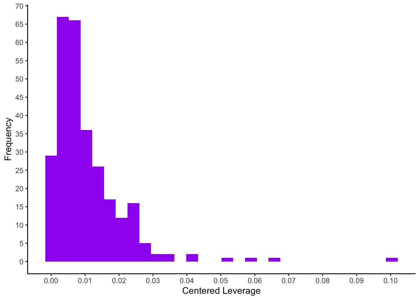
Since the recommendations for cut-offs for regression diagnostic statistics are partly inconsistent, we will use the empirical distribution (histogram) to identify persons with extreme values in the current model.
Identification of observations with high leverage values (here we select all \(\geq 0.05\)):
lifesat %>%
  filter(leveragec > 0.05)
## # A tibble: 4 × 5
## ID lifesat_overall se_assertive se_social se_relationships
## <fct> <dbl> <dbl> <dbl> <dbl>
## 1 21 3.45 1 1.57 4.83
## 2 168 4.64 2.33 5 4
## 3 283 5.18 3 6.14 5.83
## 4 313 2.91 1.33 2.57 3.83Outlier statistics on the dependent variable: residuals
Raw residuals are obtained using residuals(model) and studentized residuals via rstandard(model). The most relevant studentized deleted residuals can be obtained with rstudent(model).
We want to identify thresholds of extreme residuals, thus we will look at the 0.5%, 2.5%, 50%, 97.5% and 99.5% quantiles of all residual measures. For reasons of space we will obtain the histogram with the full distribution only for studentized deleted residuals (stud_del).
res <- residuals(model_life)
stud_res <- rstandard(model_life)
stud_del <- rstudent(model_life)

ps <- c(0, 0.005, 0.025, 0.5, 0.975, 0.995, 1)
quantile(res, ps) %>% round(3)
## 0% 0.5% 2.5% 50% 97.5% 99.5% 100%
## -2.418 -1.586 -1.014 0.000 0.951 1.152 1.194quantile(stud_res, ps) %>% round(3)## 0% 0.5% 2.5% 50% 97.5% 99.5% 100%
## -4.671 -3.075 -1.959 0.001 1.827 2.224 2.308quantile(stud_del, ps) %>% round(3)## 0% 0.5% 2.5% 50% 97.5% 99.5% 100%
## -4.855 -3.124 -1.969 0.001 1.835 2.240 2.326ggplot(mapping = aes(x = stud_del)) +
geom_histogram(fill=I("purple")) +
scale_x_continuous(breaks = seq(-5.5, 3, 0.5)) +
scale_y_continuous(breaks = seq(0, 35, 5)) +
xlab("Studentized Deleted Residual") +
ylab("Frequency") +
theme_classic()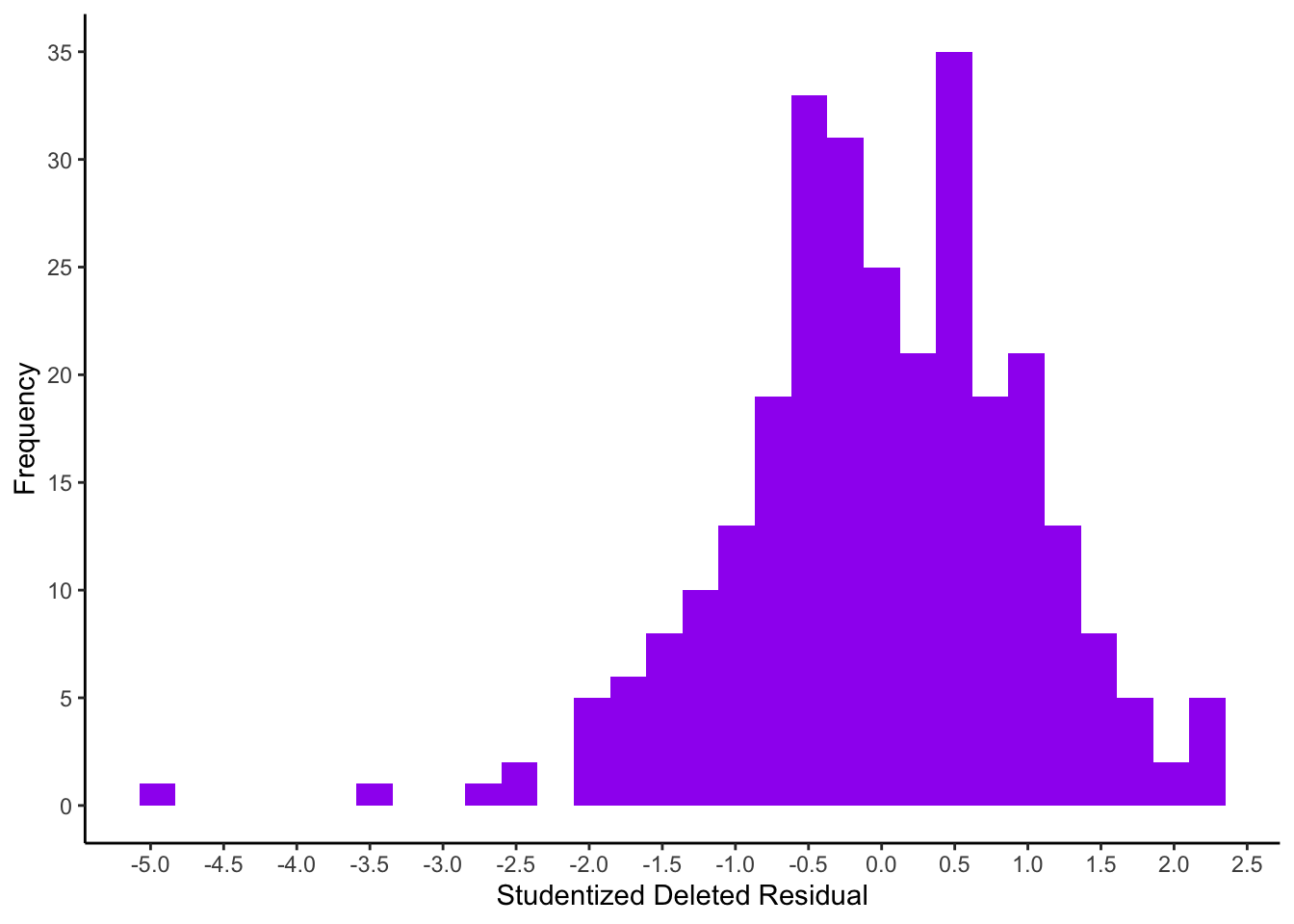
To only identify people with really large studentized deleted residuals the rule-of-thumb threshold of absolute values \(\geq 3\) (Eid, Gollwitzer, & Schmitt, 2017) is applied here.
lifesat %>%
  filter(abs(stud_del) >= 3)
## # A tibble: 2 × 5
## ID lifesat_overall se_assertive se_social se_relationships
## <fct> <dbl> <dbl> <dbl> <dbl>
## 1 60 3.27 5.33 3.86 5.17
## 2 339 3 6.33 4.71 5.67Influential data points
Influential data points for particular regression coefficients
The DfBeta values correspond to the difference between a certain regression coefficient for a model calculated including a certain person and a model calculated without this person. They can be obtained using the function dfbeta(model). However, only the standardised DfBetaS values (obtained with dfbetas(model)) can be interpreted independently of the measurement scale of the variables.
The output of dfbeta(model) and dfbetas(model) is a matrix with persons in the rows and the variables/model effects in the columns. To be able to look at the distribution of the coefficients for each predictor (se_assertive, se_social, se_relationships), the matrix must first be converted into a dataframe.
In the following the quantiles for both DfBeta and DfBetaS will be requested, but histograms will be created only for the more relevant DfBetaS:
my_dfbeta <- data.frame(dfbeta(model_life))
my_dfbetas <- data.frame(dfbetas(model_life))

quantile(my_dfbeta$se_assertive, ps) %>% round(3)
## 0% 0.5% 2.5% 50% 97.5% 99.5% 100%
## -0.020 -0.010 -0.005 0.000 0.005 0.011 0.015quantile(my_dfbetas$se_assertive, ps) %>% round(3)## 0% 0.5% 2.5% 50% 97.5% 99.5% 100%
## -0.532 -0.252 -0.130 0.001 0.135 0.288 0.376ggplot(mapping = aes(x = my_dfbetas$se_assertive)) +
geom_histogram(fill=I("darkgreen")) +
scale_x_continuous(breaks = seq(-0.5, 0.5, 0.1)) +
scale_y_continuous(breaks = seq(0, 150, 10)) +
xlab("DfBetaS se_assertive") +
ylab("Frequency") +
theme_classic()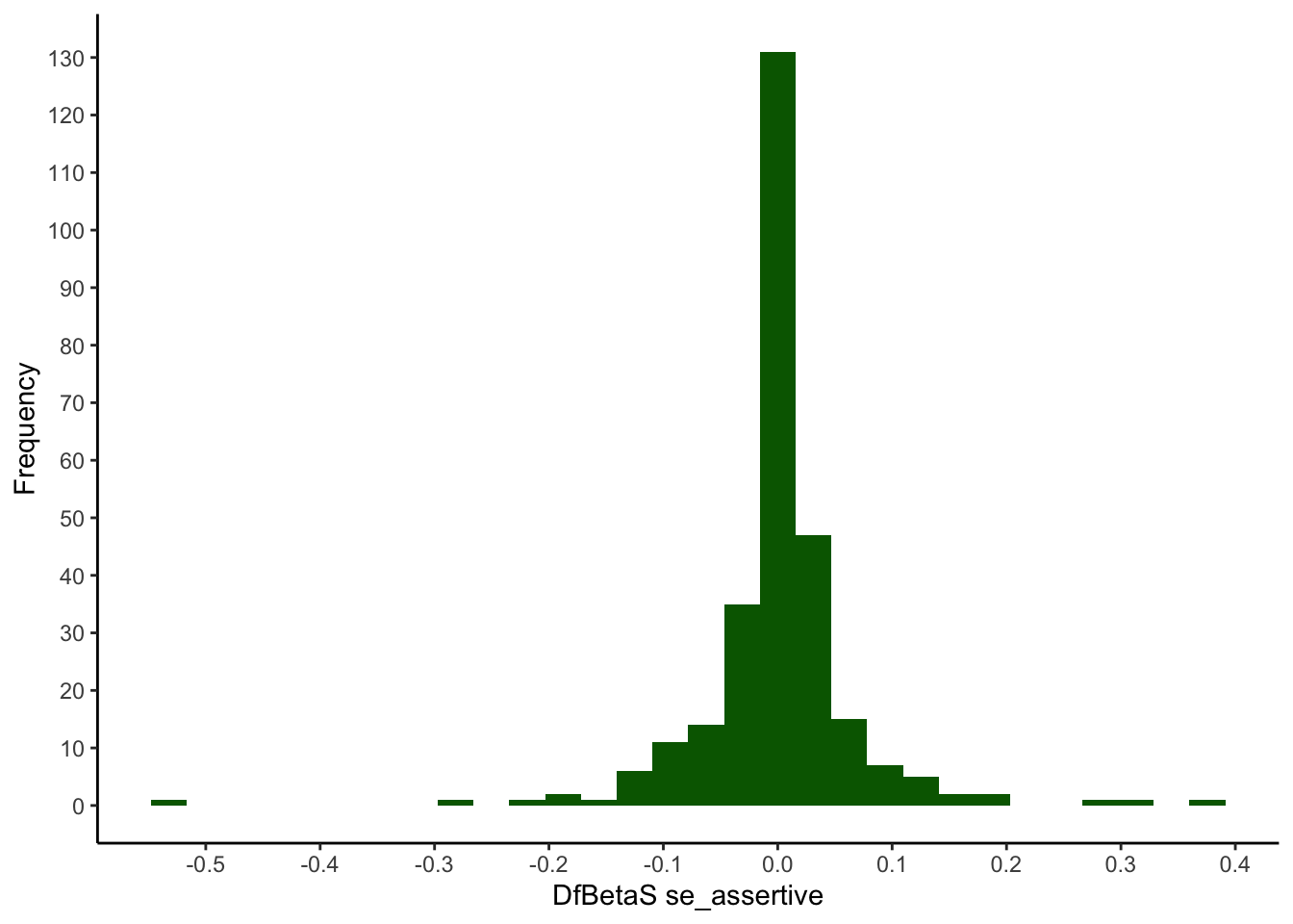
quantile(my_dfbeta$se_social, ps) %>% round(3)## 0% 0.5% 2.5% 50% 97.5% 99.5% 100%
## -0.010 -0.008 -0.005 0.000 0.006 0.020 0.025quantile(my_dfbetas$se_social, ps) %>% round(3)## 0% 0.5% 2.5% 50% 97.5% 99.5% 100%
## -0.190 -0.152 -0.100 -0.006 0.121 0.388 0.493ggplot(mapping = aes(x = my_dfbetas$se_social)) +
geom_histogram(fill=I("darkgreen")) +
scale_x_continuous(breaks = seq(-0.5, 0.5, 0.1)) +
scale_y_continuous(breaks = seq(0, 100, 5)) +
xlab("DfBetaS se_social") +
ylab("Frequency") +
theme_classic()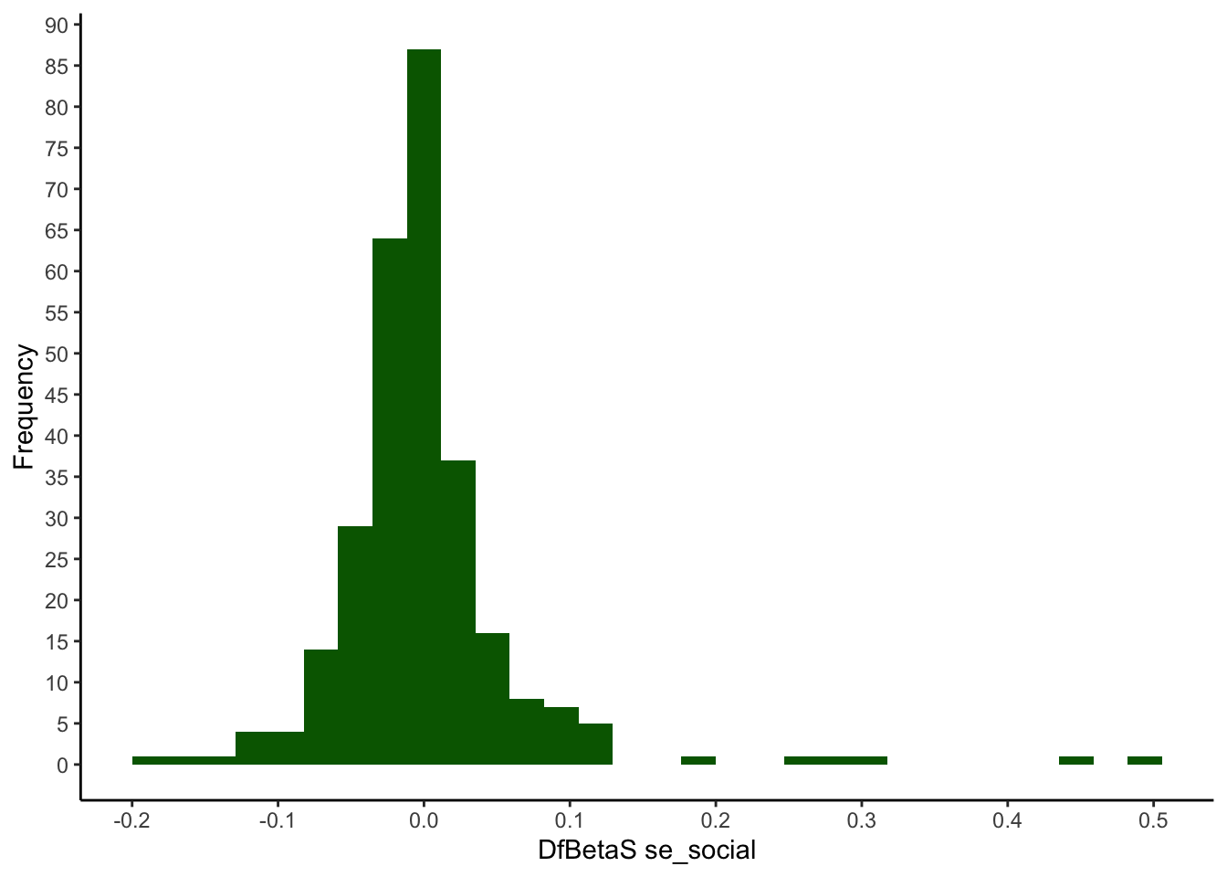
quantile(my_dfbeta$se_relationships, ps) %>% round(3)## 0% 0.5% 2.5% 50% 97.5% 99.5% 100%
## -0.014 -0.010 -0.007 0.000 0.005 0.010 0.014quantile(my_dfbetas$se_relationships, ps) %>% round(3)## 0% 0.5% 2.5% 50% 97.5% 99.5% 100%
## -0.303 -0.219 -0.147 0.000 0.111 0.219 0.288ggplot(mapping = aes(x = my_dfbetas$se_relationships)) +
geom_histogram(fill=I("darkgreen")) +
scale_x_continuous(breaks = seq(-0.5, 0.5, 0.1)) +
scale_y_continuous(breaks = seq(0, 100, 5)) +
xlab("DfBetaS se_relationships") +
ylab("Frequency") +
theme_classic()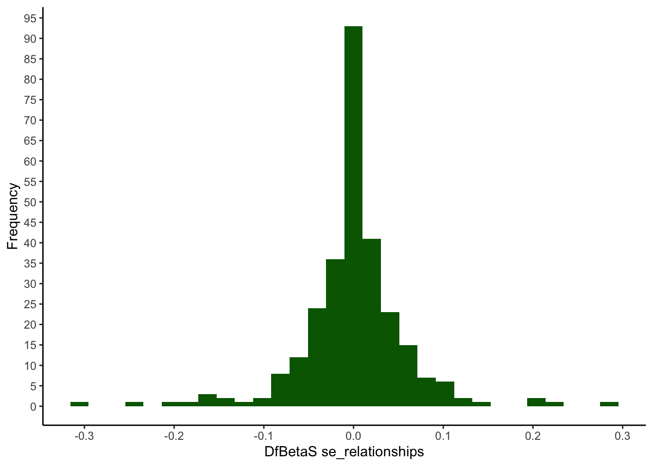
Influential data points for the overall model: DfFitS and Cook’s distance
The DfFitS (function dffits()) represents a standardized difference between a person’s predicted values from models estimated with and without the person, and the Cook’s distance (function cooks.distance()) is a further standardized measure of overall influence. Since they are a function of the squared DfFitS, Cook’s distances cannot be negative.
my_dffits <- dffits(model_life)
quantile(my_dffits, ps) %>% round(3)
## 0% 0.5% 2.5% 50% 97.5% 99.5% 100%
## -0.656 -0.544 -0.311 0.000 0.216 0.314 0.338ggplot(mapping = aes(x = my_dffits)) +
geom_histogram(fill=I("darkblue")) +
scale_x_continuous(breaks = seq(-1, 1, 0.1)) +
scale_y_continuous(breaks = seq(0, 100, 5)) +
xlab("DfFitS") +
ylab("Frequency") +
theme_classic()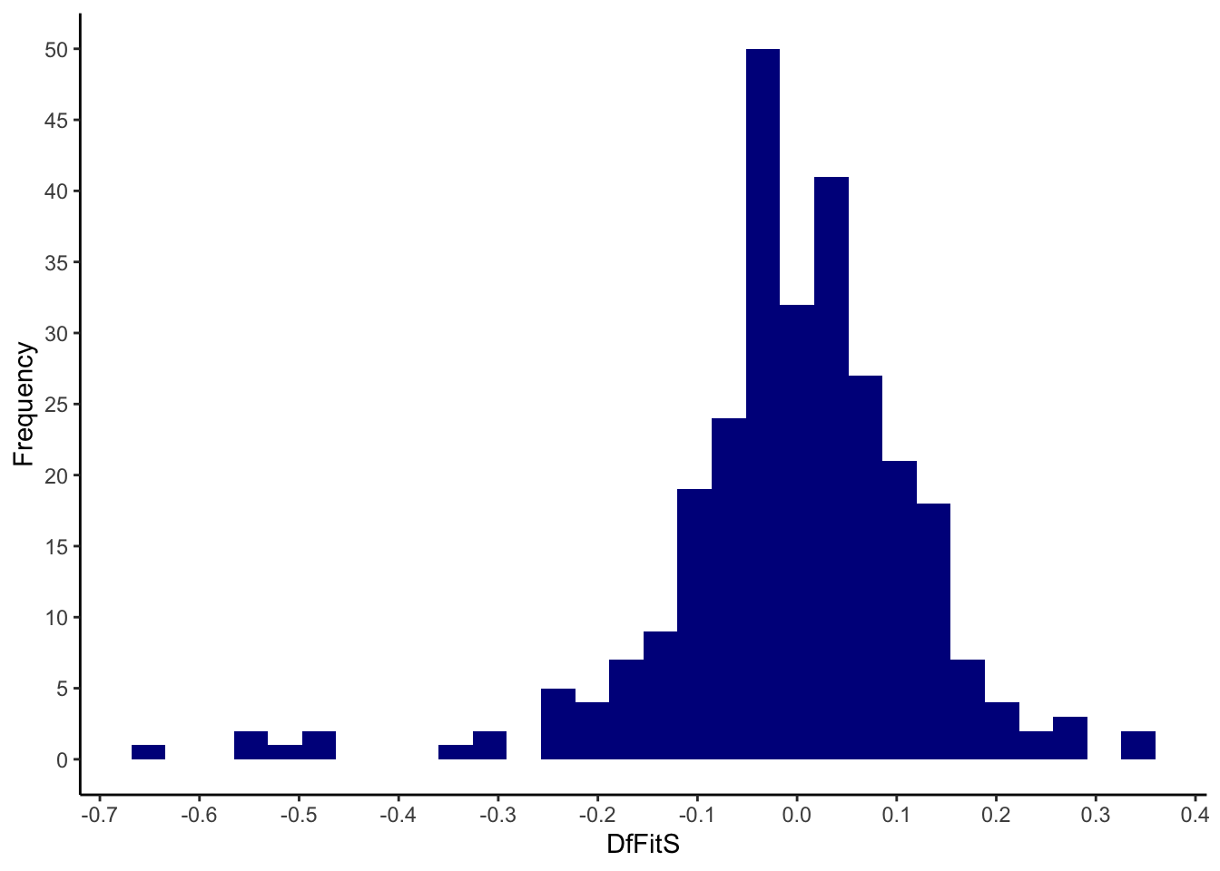
Let’s look at the Cook’s distances:
my_cooks <- cooks.distance(model_life)
quantile(my_cooks, p = c(0, 0.5, 0.95, 0.99, 1)) %>% round(3)
## 0% 50% 95% 99% 100%
## 0.000 0.001 0.016 0.064 0.100ggplot(mapping = aes(x = my_cooks)) +
geom_histogram(fill=I("darkblue")) +
scale_x_continuous(breaks = seq(0, 1, 0.01)) +
scale_y_continuous(breaks = seq(0, 150, 10)) +
xlab("Cook's Distance") +
ylab("Frequency") +
theme_classic()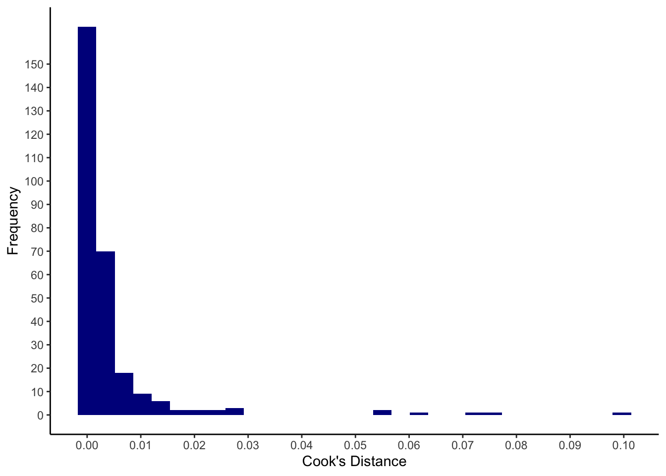
To identify only observations with substantial Cook’s distances, we consider those with an absolute value \(\geq 0.07\) (cut-off determined ad hoc):
lifesat %>%
  filter(my_cooks >= 0.07)
## # A tibble: 3 × 5
## ID lifesat_overall se_assertive se_social se_relationships
## <fct> <dbl> <dbl> <dbl> <dbl>
## 1 21 3.45 1 1.57 4.83
## 2 313 2.91 1.33 2.57 3.83
## 3 339 3 6.33 4.71 5.67These are the persons with the IDs 21, 313 and 339.
A representation for identifying the most influential data points via Cook’s Distance can be obtained using the plot() function on the model object together with the selection argument which = 4.
plot(model_life, labels.id = lifesat$ID, which = 4)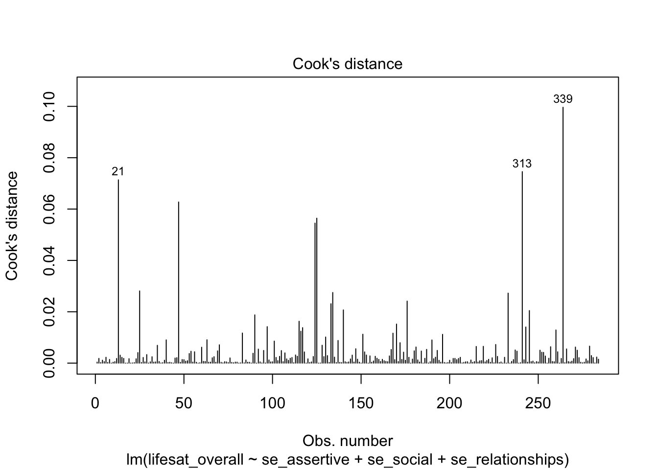
The labels.id argument can be used to specify the variable whose values will be used to identify the most prominent values in the diagram (IDs 21, 313 and 319 that we also identified as “conspicuous”).
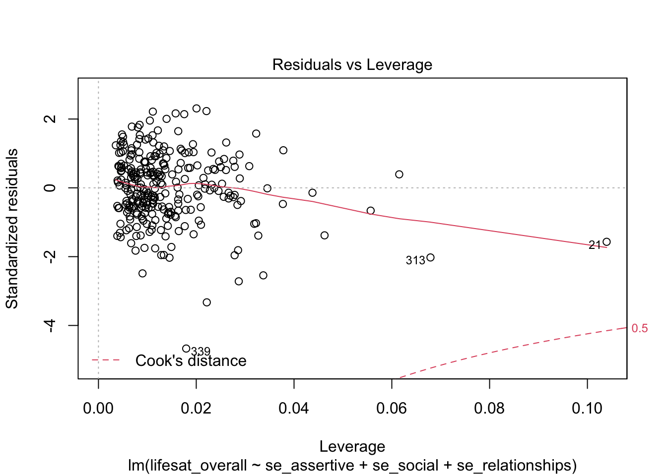
Using the selection argument which = 5 we obtain a “Residuals vs Leverage Plot” with the leverage values on the x axis and the studentized residuals on the y axis.
plot(model_life, labels.id = lifesat$ID, which = 5)
A (dashed) line is drawn with the Cook’s Distance limit of 0.5 (this limit is used here independent of the data situation). In our case this limit is within the plot display area only for the negative residuals. No observed value exceeds this limit (we already know this). For the positive residuals this limit also exists, it is just not visible here, because there is no positive residual value near this limit. This plot shows that those values have the greatest influence on the model whose combination of leverage and residual is the greatest.
Estimating the model without the identified influential data points
lifesat_red <- lifesat %>%
  filter(my_cooks < 0.07)

model_life2 <- lm(lifesat_overall ~ se_assertive + se_social + se_relationships,
             data = lifesat_red)
summary(model_life2)
##
## Call:
## lm(formula = lifesat_overall ~ se_assertive + se_social + se_relationships,
## data = lifesat_red)
##
## Residuals:
## Min 1Q Median 3Q Max
## -1.80261 -0.29631 -0.00773 0.32401 1.19833
##
## Coefficients:
## Estimate Std. Error t value Pr(>|t|)
## (Intercept) 1.88028 0.26190 7.179 6.46e-12 ***
## se_assertive 0.05787 0.03821 1.515 0.1310
## se_social 0.10228 0.05208 1.964 0.0505 .
## se_relationships 0.48231 0.04541 10.621 < 2e-16 ***
## ---
## Signif. codes: 0 '***' 0.001 '**' 0.01 '*' 0.05 '.' 0.1 ' ' 1
##
## Residual standard error: 0.4974 on 277 degrees of freedom
## Multiple R-squared: 0.4256, Adjusted R-squared: 0.4194
## F-statistic: 68.42 on 3 and 277 DF, p-value: < 2.2e-16After exclusion of the most influential data points (Cook’s Distance \(\ge 0.07\): IDs 21, 313, 339) the effect of se_social is no longer significant. The effects of the two other predictors remain unchanged.
Inspecting the values of the excluded persons on the IV se_social (\(\bar x = 5.418\)) as well as the DV lifesat_overall (\(\bar x = 5.278)\), it becomes clear that all three persons reported both a below-average se_social and a very low lifesat_overall, reflecting a positive correlation between the two variables. For the remaining 281 persons, however, there seems to be hardly any (unique) predictive contribution of se_social for lifesat_overall.
lifesat %>%
  filter(my_cooks >= 0.07)
## # A tibble: 3 × 5
## ID lifesat_overall se_assertive se_social se_relationships
## <fct> <dbl> <dbl> <dbl> <dbl>
## 1 21 3.45 1 1.57 4.83
## 2 313 2.91 1.33 2.57 3.83
## 3 339 3 6.33 4.71 5.67It is very difficult to argue that specific observations should be excluded from a model based on an analysis of influential data points. However, in any case, these kind of residual diagnostics can help us understand our data and results better.
9.4.3 Homoscedasticity
The homoscedasticity assumption can be tested by inspecting the distribution of the residuals over the range of the predicted values. If the residuals scatter equally (around 0) at all points of the predicted values, homoscedasticity is given. A graph can be obtained with the plot() function and the selection argument which = 1.
plot(model_life, labels.id = lifesat$ID, which = 1)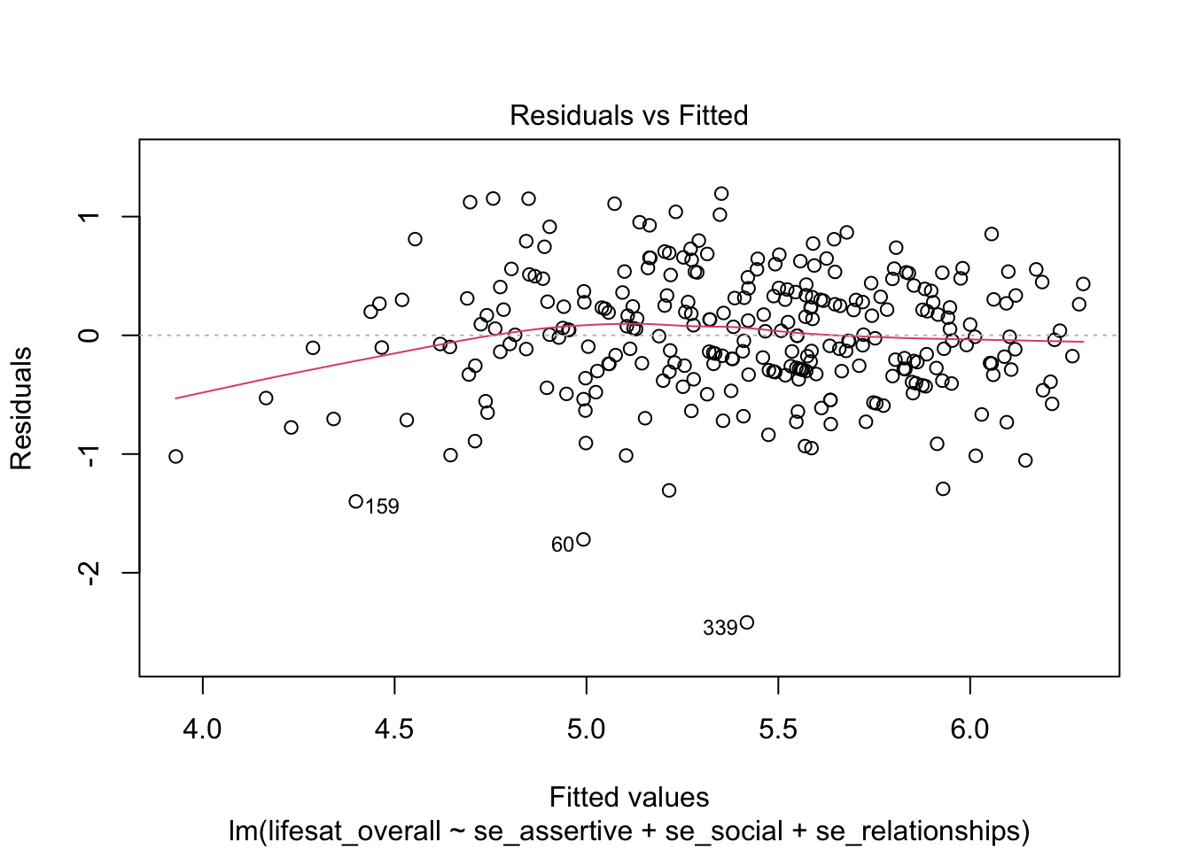
This plot shows quite nicely that the distribution of residuals is very similar over the range of fitted values. It can also be used to check the correct specification of the model in terms of the linearity assumption: The residuals should have a mean value of 0 across the whole range of predicted values. This is also the case here (red line).
9.4.4 Normality of residuals
The normality assumption can be checked using a quantile-quantile-plot (QQ-plot), which is obtained using plot() and which = 2:
plot(model_life, labels.id = lifesat$ID, which = 2)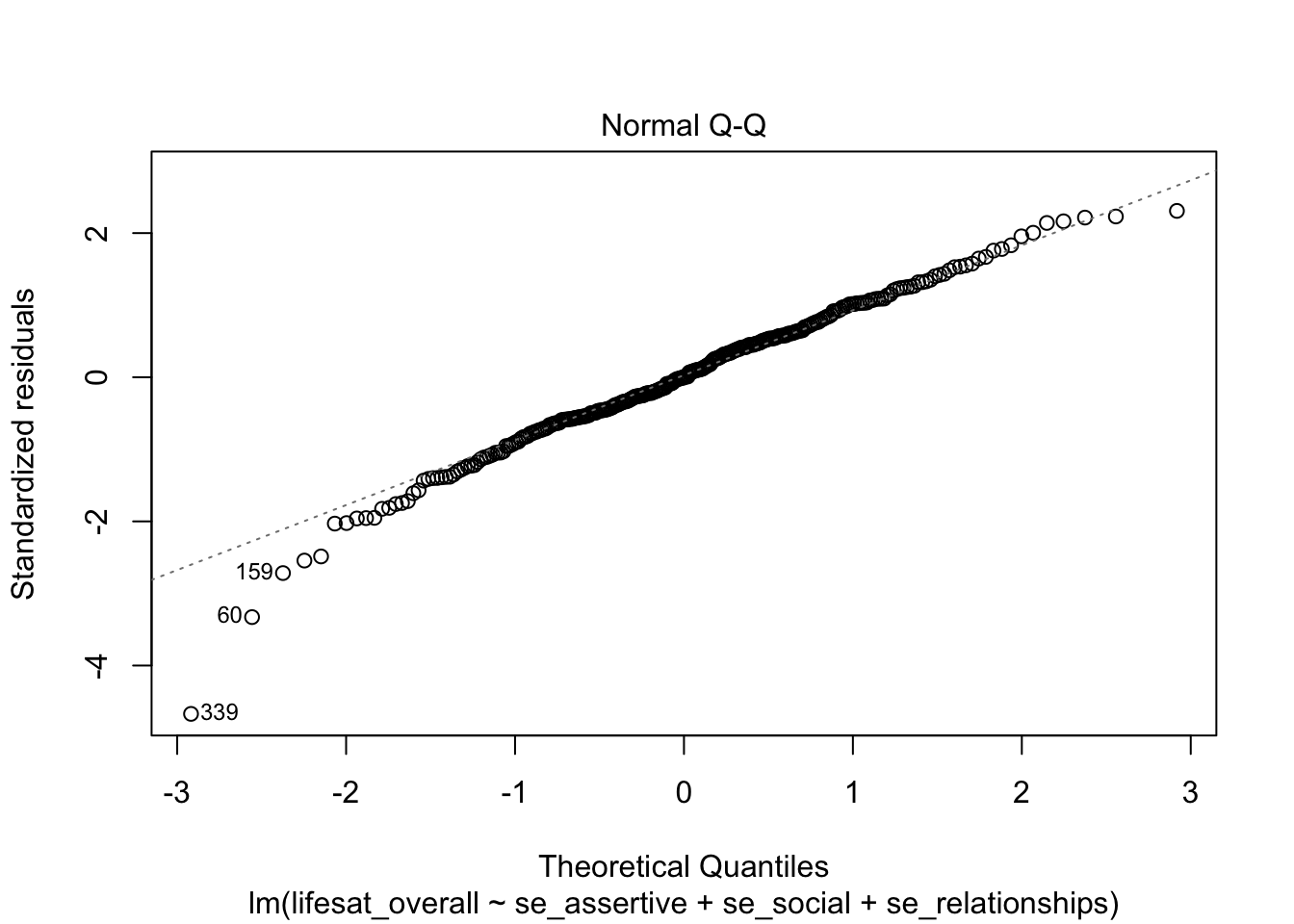
On the x axis the theoretical normal distribution quantiles are plotted, on the y axis the studentized residuals. If the residuals are normally distributed, the empirical residuals should have the same value as the corresponding z quantile. Here, the person with ID = 339 has a studentized residual of < -4, although he/she should have a value of -3 at most (in terms of the expected normal distribution of the residuals).
Except for a few outliers the residuals seem to be normally distributed.
9.4.5 Diagnostic graphics at a glance
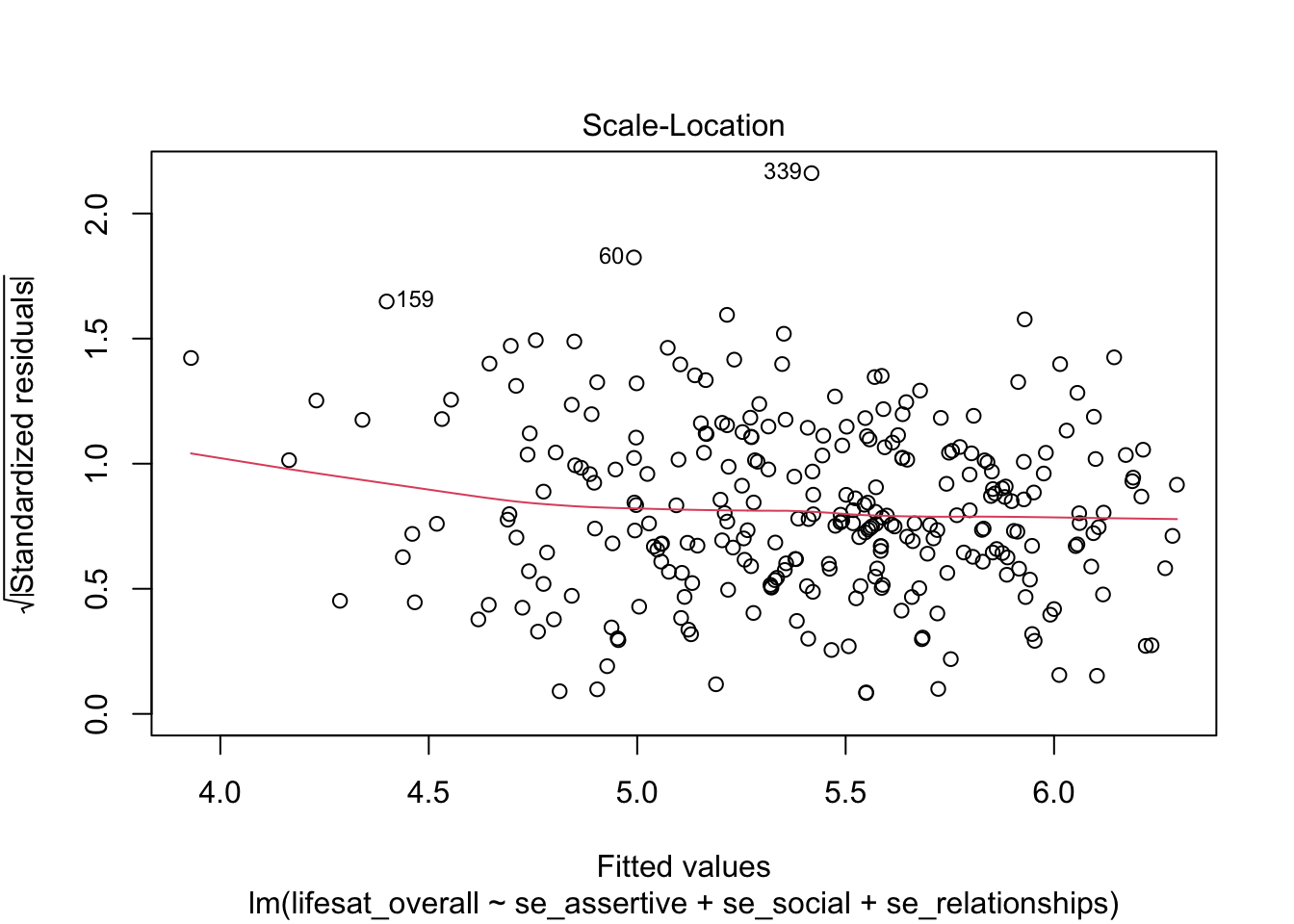
When using the plot() function without the which argument a plot of four diagnostic graphics is obtained, three of which we already know. An additional plot is the third plot (which = 3) that may be used for a more fine-grained analysis of the homoscadasticity assumption. Here, the square root of the absolute values of the standardized residuals are plotted against the fitted values. This allows to asses the average absolute value of residuals (red line). If this value is similar across the range of fitted values, the residuals have similar variance and thus homoscedasticity is given.
plot(model_life, labels.id = lifesat$ID)

9.4.6 Regression diagnostics conclusions
Overall, our regression diagnostics have shown that the assumptions of the regression model are largely met. However, there are some data points that affect the normal distribution of the residuals and show partly conspicuous values in the statistics for influential data points. An alternative model has shown that without the six most influential observations, only the variable se_relationships was a significant predictor for lifesat_overall, whereas in the original model, se_social also had a significant effect on life satisfaction.
In any case, the exclusion of observations based on regression diagnostics must be very well justified. Only if the conspicuous values are obvious mistakes or if the participants obviously did not answer seriously (e.g, uniform response patterns), can these observations/persons be excluded without further ado.
9.5 Moderated regression analysis
A moderation analysis is typically represented by a regression equation containing the main effects of the focal predictor (support_parents), the moderator (se_social) and the interaction term (product variable):
\(Y = b_0 + b_1 \cdot X_1 + b_2 \cdot X_2 + b_3 \cdot X_1 \cdot X_2 + E\)
Statistically the focal predictor and the moderator are exchangeable, but conceptually they should be always explicitly differentiated. We can represent the equation also in its conditional effect form where the focal predictor (here: \(X_1\)) is put outside the brackets:
\(Y = (b_0 + b_2 \cdot X_2) + (b_1 + b_3 \cdot X_2) \cdot X_1 + E\)
Using the lm() formula notation such a model is specified by lm(Y ~ X1*X2, data = mydata) or by lm(Y ~ X1 + X2 + X1:X2, data = mydata)
Example: Self-efficacy as a moderator of the support \(\Rightarrow\) life satisfaction relation
We assume that the perceived emotional support by parents (support_parents) has a positive effect on life satisfaction (lifesat_overall). Young people who feel supported should be more satisfied with their lives than those who receive less emotional support from their parents.
Furthermore, we assume that social self-efficacy (se_social) moderates this effect: emotional support by parents could play a more important role for those adolescents’ life satisfaction who are rather low in social self-efficacy. On the other hand, for those with high social self-efficacy support from parents may not be that fundamental for their life satisfaction since they may experience more support from peers.
The statistical moderation hypothesis is therefore:
“The higher adolescents’ social self-efficacy, the weaker the effect of parental emotional support on their life satisfaction.” Thus, a negative interaction effect of support_parents \(\times\) se_social is expected.
For average socially self-effective adolescents (“Mean”), a positive effect of parental support on life satisfaction is expected (since we also expect an overall positive effect).
The positive effect should be stronger for young people with below-average social self-efficacy (- 1 SD) and weaker for young people with above-average social-self-efficacy (+ 1 SD).
Data:
mod <- adolescents %>%
  dplyr::select(support_parents, lifesat_overall, se_social) %>%
  drop_na()

head(mod)
## # A tibble: 6 × 3
## support_parents lifesat_overall se_social
## <dbl> <dbl> <dbl>
## 1 6.67 5.91 5.14
## 2 5.17 4.64 5.57
## 3 6.83 5.18 5.43
## 4 7 5.82 6
## 5 6.67 5.82 4.8
## 6 6.5 5.36 4.71describe(mod, fast = TRUE)## vars n mean sd min max range se
## support_parents 1 284 5.87 1.00 1.50 7.00 5.50 0.06
## lifesat_overall 2 284 5.42 0.69 2.91 6.91 4.00 0.04
## se_social 3 284 5.28 0.79 1.57 7.00 5.43 0.059.5.1 Estimating the moderated regression model
modreg <- lm(lifesat_overall ~ support_parents*se_social, data = mod)
summary(modreg)
##
## Call:
## lm(formula = lifesat_overall ~ support_parents * se_social, data = mod)
##
## Residuals:
## Min 1Q Median 3Q Max
## -1.66104 -0.33321 0.00913 0.39591 1.09442
##
## Coefficients:
## Estimate Std. Error t value Pr(>|t|)
## (Intercept) -0.48129 0.92134 -0.522 0.60182
## support_parents 0.74178 0.16280 4.557 7.77e-06 ***
## se_social 0.77313 0.17776 4.349 1.91e-05 ***
## support_parents:se_social -0.08138 0.03089 -2.635 0.00889 **
## ---
## Signif. codes: 0 '***' 0.001 '**' 0.01 '*' 0.05 '.' 0.1 ' ' 1
##
## Residual standard error: 0.5195 on 280 degrees of freedom
## Multiple R-squared: 0.4428, Adjusted R-squared: 0.4369
## F-statistic: 74.18 on 3 and 280 DF, p-value: < 2.2e-16The interaction is significant and negative, thus in line with our moderation hypothesis. An increase of the moderator se_social by one unit leads to a \(b_3= -0.081\) lower effect of support_parents on lifesat_overall. Thus, for socially more self-efficacious adolescents the influence of parental support on life satisfaction was significantly lower than for socially less self-effective adolescents.
Another (slightly more complicated) possibility of calculation is to first estimate a model with the two predictors as main effects (multiple regression) and then to add the interaction effect in an additional model. A model comparison then can test the significance of the interaction effect. This procedure is actually not needed here since the interaction effect is estimated by a single parameter and thus the model comparison F test is equivalent to the t test of the interaction term.
# Model without interaction
multreg <- lm(lifesat_overall ~ support_parents + se_social, data = mod)

# Add interaction term using update()
modreg <- update(multreg, . ~ . + support_parents:se_social, data = mod)

# Model comparison
anova(multreg, modreg)
## Analysis of Variance Table
##
## Model 1: lifesat_overall ~ support_parents + se_social
## Model 2: lifesat_overall ~ support_parents + se_social + support_parents:se_social
## Res.Df RSS Df Sum of Sq F Pr(>F)
## 1 281 77.453
## 2 280 75.580 1 1.8737 6.9414 0.008891 **
## ---
## Signif. codes: 0 '***' 0.001 '**' 0.01 '*' 0.05 '.' 0.1 ' ' 19.5.2 Moderated regression with centered predictors
Calculating the moderated regression analysis with centered predictor variables has the advantage that the main effect of the focal predictor variable (support_parents_c) corresponds to the conditional effect (simple slope) at the mean of the moderator variable (= at position 0 of the centered moderator variable se_social_c).
Centering the predictors:
mod <- mod %>%
  mutate(support_parents_c = support_parents - mean(support_parents),
         se_social_c = se_social - mean(se_social))

# Alternatively using the scale() function
mod <- mod %>%
  mutate(support_parents_c = scale(support_parents, scale = FALSE),
         se_social_c = scale(se_social, scale = FALSE))

describe(mod, fast = TRUE)
## vars n mean sd min max range se
## support_parents 1 284 5.87 1.00 1.50 7.00 5.50 0.06
## lifesat_overall 2 284 5.42 0.69 2.91 6.91 4.00 0.04
## se_social 3 284 5.28 0.79 1.57 7.00 5.43 0.05
## support_parents_c 4 284 0.00 1.00 -4.37 1.13 5.50 0.06
## se_social_c 5 284 0.00 0.79 -3.71 1.72 5.43 0.05Calculate the moderated regression with the centered variables:
modreg_c <- lm(lifesat_overall ~ support_parents_c*se_social_c, data = mod)
summary(modreg_c)
##
## Call:
## lm(formula = lifesat_overall ~ support_parents_c * se_social_c,
## data = mod)
##
## Residuals:
## Min 1Q Median 3Q Max
## -1.66104 -0.33321 0.00913 0.39591 1.09442
##
## Coefficients:
## Estimate Std. Error t value Pr(>|t|)
## (Intercept) 5.43324 0.03143 172.858 < 2e-16 ***
## support_parents_c 0.31202 0.03213 9.710 < 2e-16 ***
## se_social_c 0.29530 0.04151 7.114 9.43e-12 ***
## support_parents_c:se_social_c -0.08138 0.03089 -2.635 0.00889 **
## ---
## Signif. codes: 0 '***' 0.001 '**' 0.01 '*' 0.05 '.' 0.1 ' ' 1
##
## Residual standard error: 0.5195 on 280 degrees of freedom
## Multiple R-squared: 0.4428, Adjusted R-squared: 0.4369
## F-statistic: 74.18 on 3 and 280 DF, p-value: < 2.2e-16The simple slope of the focal predictor variable at the mean value of the moderator variable is \(b_{mean} = 0.312\) and this effect is significant (\(p = 0\)).
9.5.3 Simple slopes and plots with interactions
With sim_slopes() the simple slopes of the focal predictor can be tested and plotted at any value of the moderator. By default, simple slopes at the mean as well as +/- 1 SD from the mean of the moderator variable are computed:
library(interactions)
sim_slopes(modreg, pred = "support_parents", modx = "se_social",
           johnson_neyman = FALSE)
## SIMPLE SLOPES ANALYSIS
##
## Slope of support_parents when se_social = 4.495525 (- 1 SD):
##
## Est. S.E. t val. p
## ------ ------ -------- ------
## 0.38 0.04 9.87 0.00
##
## Slope of support_parents when se_social = 5.280659 (Mean):
##
## Est. S.E. t val. p
## ------ ------ -------- ------
## 0.31 0.03 9.71 0.00
##
## Slope of support_parents when se_social = 6.065793 (+ 1 SD):
##
## Est. S.E. t val. p
## ------ ------ -------- ------
## 0.25 0.04 5.86 0.00Specific moderator values can be specified using the modx.values argument. Like this, for example, we can obtain the simple slopes for the minimum and maximum values of the moderator:
sim_slopes(modreg, pred = "support_parents", modx = "se_social",
           modx.values = c(1.57143, 7), johnson_neyman = FALSE)
## SIMPLE SLOPES ANALYSIS
##
## Slope of support_parents when se_social = 1.57143:
##
## Est. S.E. t val. p
## ------ ------ -------- ------
## 0.61 0.12 5.31 0.00
##
## Slope of support_parents when se_social = 7.00000:
##
## Est. S.E. t val. p
## ------ ------ -------- ------
## 0.17 0.06 2.65 0.01The resulting simple slopes are \(b_{min} = 0.61\) and \(b_{max} = 0.17\), and both are significant.
interact_plot() provides a graphic depiction of the simple slopes at the mean and mean +/- 1 SD:
interact_plot(modreg, pred = "support_parents", modx = "se_social",
              x.label = "Support by Parents",
              y.label = "Life Satisfaction",
              legend.main = "Social Self-Efficacy",
              colors = "Greens")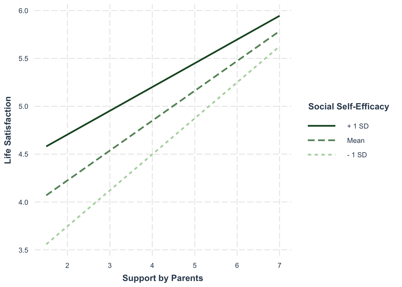
Finally, johnson_neyman() can be used to obtain the Regions of Significance (Johnson-Neyman Interval, JNI):
johnson_neyman(modreg, pred = "support_parents", modx = "se_social",
               alpha = 0.05)
## JOHNSON-NEYMAN INTERVAL
##
## When se_social is OUTSIDE the interval [7.33, 20.88], the slope of
## support_parents is p < .05.
##
## Note: The range of observed values of se_social is [1.57, 7.00]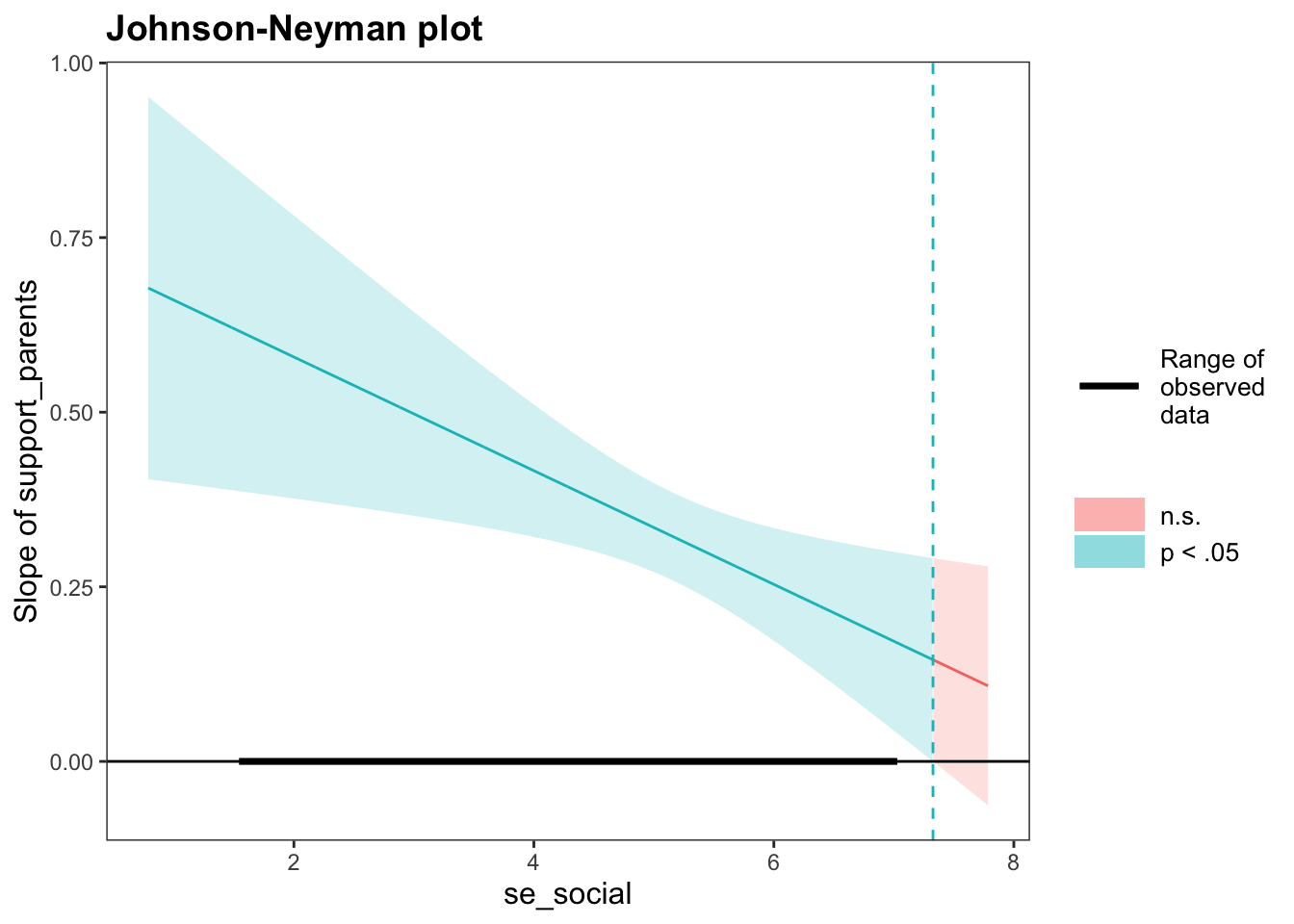
For all moderator values \([1.57, 7.00]\) existing in this dataset, the simple slope of support_parents was positively significant at the \(\alpha = 0.05\) level, since all these values are OUTSIDE the \(JNI = [7.33, 20.88]\). Since the moderator values specified in the JNI do not exist (because the moderator was measured on a scale of 1-7), the values specified here are irrelevant in a practical sense.
9.6 Analysis of non-linear effects using linear regression
Non-linear effects of predictors can be analyzed in the linear regression framework by adding polynomial (quadratic, cubic etc.) terms to the regression equation:
\(Y = b_0 + b_1 \cdot X + b_2 \cdot X^2 + b_3 \cdot X^3 + E\)
9.6.1 Quadratic effect of academic self-efficacy on stress symptoms
Let us assume that both an extremely low and a very high academic self-efficacy may be associated with increased stress symptoms, while a medium level may be associated with fewer stress symptoms.
The assumption is based on the everyday-observation that people with very high achievement motivation are often under a particular (self-imposed) pressure that can lead to increased psychosomatic stress. Furthermore, it can be assumed that very low self-efficacy will also associated with increased stress symptoms.
The hypothesized U-shaped relationship reflects a positive quadratic effect of
se_achievement on stress_soma.
Data:
nonlin <- adolescents %>%
  dplyr::select(ID, stress_soma, se_achievement) %>%
  drop_na()

head(nonlin)
## # A tibble: 6 × 3
## ID stress_soma se_achievement
## <fct> <dbl> <dbl>
## 1 1 3 4.57
## 2 2 3.83 5
## 3 10 3.33 5
## 4 11 3.5 4.57
## 5 12 1.33 5.33
## 6 14 1.5 4.86describe(nonlin[,-1], fast = TRUE)## vars n mean sd min max range se
## stress_soma 1 283 3.02 1.19 1.00 7 6.00 0.07
## se_achievement 2 283 5.09 0.77 2.43 7 4.57 0.059.6.2 Estimating the regression for a quadratic effect
To estimate the quadratic effect (DV: stress_somatisch), we have to first calculate a squared IV se_achievement_2:
nonlin <- nonlin %>%
  mutate(se_achievement_2 = se_achievement^2)

head(nonlin)
## # A tibble: 6 × 4
## ID stress_soma se_achievement se_achievement_2
## <fct> <dbl> <dbl> <dbl>
## 1 1 3 4.57 20.9
## 2 2 3.83 5 25
## 3 10 3.33 5 25
## 4 11 3.5 4.57 20.9
## 5 12 1.33 5.33 28.4
## 6 14 1.5 4.86 23.6Let’s calculate a hierarchical regression model with only the predictor se_achievement in the first model and the additional predictor se_achievement_2 in the second model. This means that the first model contains only the linear term, while the second model contains both the linear and the quadratic term.
Are the two models significant? How do the \(R^2\) of the two models differ?
Is the quadratic effect in the second model significant? Direction of the effect? Additionally, let’s perform a model comparison with anova().
linreg <- lm(stress_soma ~ se_achievement, data = nonlin)
summary(linreg)
##
## Call:
## lm(formula = stress_soma ~ se_achievement, data = nonlin)
##
## Residuals:
## Min 1Q Median 3Q Max
## -2.1164 -0.8121 -0.0874 0.6879 4.1734
##
## Coefficients:
## Estimate Std. Error t value Pr(>|t|)
## (Intercept) 3.53663 0.47590 7.431 1.3e-12 ***
## se_achievement -0.10144 0.09245 -1.097 0.273
## ---
## Signif. codes: 0 '***' 0.001 '**' 0.01 '*' 0.05 '.' 0.1 ' ' 1
##
## Residual standard error: 1.191 on 281 degrees of freedom
## Multiple R-squared: 0.004266, Adjusted R-squared: 0.0007228
## F-statistic: 1.204 on 1 and 281 DF, p-value: 0.2735nonlinreg <- update(linreg, . ~ . + se_achievement_2)
summary(nonlinreg)##
## Call:
## lm(formula = stress_soma ~ se_achievement + se_achievement_2,
## data = nonlin)
##
## Residuals:
## Min 1Q Median 3Q Max
## -2.5549 -0.8220 -0.0865 0.6608 4.1156
##
## Coefficients:
## Estimate Std. Error t value Pr(>|t|)
## (Intercept) 8.99909 2.11824 4.248 2.93e-05 ***
## se_achievement -2.32568 0.84589 -2.749 0.00636 **
## se_achievement_2 0.22113 0.08361 2.645 0.00863 **
## ---
## Signif. codes: 0 '***' 0.001 '**' 0.01 '*' 0.05 '.' 0.1 ' ' 1
##
## Residual standard error: 1.179 on 280 degrees of freedom
## Multiple R-squared: 0.02854, Adjusted R-squared: 0.0216
## F-statistic: 4.113 on 2 and 280 DF, p-value: 0.01736anova(linreg, nonlinreg)## Analysis of Variance Table
##
## Model 1: stress_soma ~ se_achievement
## Model 2: stress_soma ~ se_achievement + se_achievement_2
## Res.Df RSS Df Sum of Sq F Pr(>F)
## 1 281 398.83
## 2 280 389.11 1 9.7219 6.9958 0.008631 **
## ---
## Signif. codes: 0 '***' 0.001 '**' 0.01 '*' 0.05 '.' 0.1 ' ' 1The linear trend in model 1 (linreg) is not significant with \(b_1= -0.101, p=0.273\). For model 2 (nonlinreg) both the overall model test is significant with \(R^2 = 0.029, F_{(2, 280)}=4.113, p=0.017\), as well as the test for the quadratic term (variable: se_achievement_2) with \(b_2=0.221, p=0.009\).
The positive quadratic term indicates that there is a U-shaped relationship as we assumed.
There is a simpler way to perform the same analysis with the advantage that the quadratic/polynomial term can be entered without explicitly computing a quadratic predictor variable:
nonlinreg1 <- lm(stress_soma ~ se_achievement + I(se_achievement^2),
                 data = nonlin)
summary(nonlinreg1)
##
## Call:
## lm(formula = stress_soma ~ se_achievement + I(se_achievement^2),
## data = nonlin)
##
## Residuals:
## Min 1Q Median 3Q Max
## -2.5549 -0.8220 -0.0865 0.6608 4.1156
##
## Coefficients:
## Estimate Std. Error t value Pr(>|t|)
## (Intercept) 8.99909 2.11824 4.248 2.93e-05 ***
## se_achievement -2.32568 0.84589 -2.749 0.00636 **
## I(se_achievement^2) 0.22113 0.08361 2.645 0.00863 **
## ---
## Signif. codes: 0 '***' 0.001 '**' 0.01 '*' 0.05 '.' 0.1 ' ' 1
##
## Residual standard error: 1.179 on 280 degrees of freedom
## Multiple R-squared: 0.02854, Adjusted R-squared: 0.0216
## F-statistic: 4.113 on 2 and 280 DF, p-value: 0.017369.6.3 Plotting the quadratic regression using ggplot2
p <- nonlin %>%
  ggplot(aes(x = se_achievement, y = stress_soma))

p + geom_jitter(width = 0.1, alpha = 0.5) +
  geom_line(aes(y = predict(nonlinreg)), size = 1, colour = "blue") +
  theme_bw()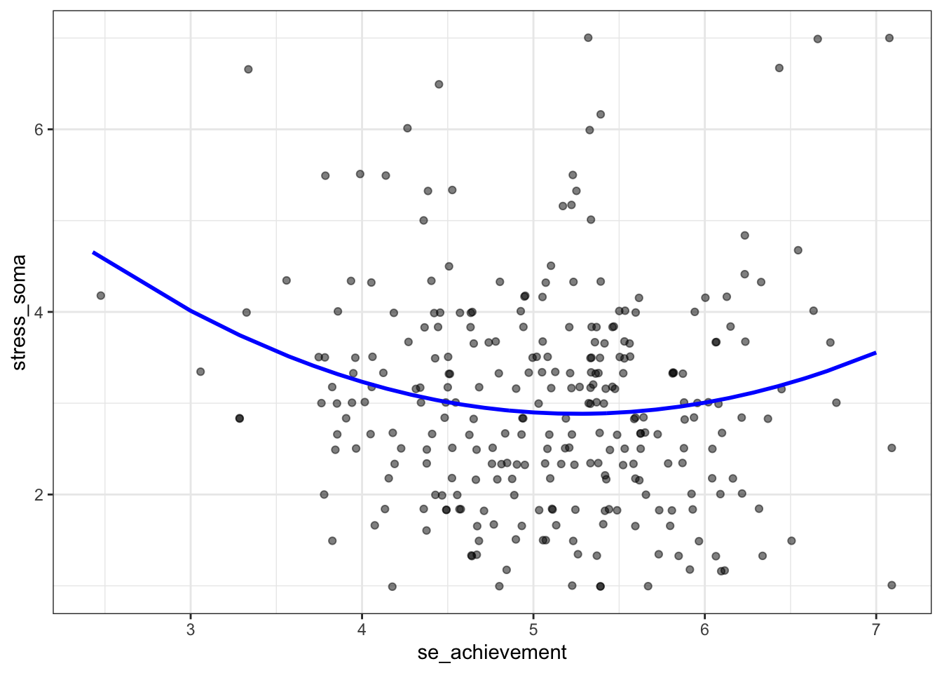
9.7 Regression with categorical predictors using dummy and effect coding
Example: Mother’s education affects adolescents’ grade average
While we looked at the effect of father’s education on adolescents grade average when introducing ANOVAs we now turn to the effect of mother’s education for grade_overall, but this time in a regression framework using categorical predictors!
Educational research shows that educational success is partly determined by the educational level of the family of origin. Therefore, we want to investigate the influence of the educational level of the mothers on adolescents’ grade average.
The hypothesis is that adolescents whose mothers have a higher educational level have better segrade than adolescents whose mothers have a lower educational level. We treat the 4-step educational level of the mother (edu_mother) as a categorical variable (factor), using only the nominal information of this ordinal variable for the analysis.
Data:
edu <- adolescents %>%
    dplyr::select(ID, grade_overall, edu_mother) %>%
    drop_na()

head(edu)
## # A tibble: 6 × 3
## ID grade_overall edu_mother
## <fct> <dbl> <fct>
## 1 2 4 Realschule
## 2 10 5 Hauptschule
## 3 11 4 Hochschule
## 4 12 5 Realschule
## 5 14 4 Realschule
## 6 15 4 Realschuletable(edu$edu_mother)##
## Hauptschule Realschule Abitur Hochschule
## 42 95 49 81Let’s first compute the mean values of grade average per category:
edu %>%
  group_by(edu_mother) %>%
  summarise(mean_grade_overall = mean(grade_overall))
## # A tibble: 4 × 2
## edu_mother mean_grade_overall
## <fct> <dbl>
## 1 Hauptschule 4.10
## 2 Realschule 4.37
## 3 Abitur 4.49
## 4 Hochschule 4.729.7.1 Regression with dummy coded categorical predictors
There are several ways to dummy code a categorical variable in R. The first (though not the simplest) possibility we look at is using dummy.code() from the psych package:
dummies <- psych::dummy.code(edu$edu_mother) # creates dummy variables
edu <- data.frame(edu, dummies) # adds dummy variables to the data frame

head(edu)
## ID grade_overall edu_mother Realschule Hochschule Abitur Hauptschule
## 1 2 4 Realschule 1 0 0 0
## 2 10 5 Hauptschule 0 0 0 1
## 3 11 4 Hochschule 0 1 0 0
## 4 12 5 Realschule 1 0 0 0
## 5 14 4 Realschule 1 0 0 0
## 6 15 4 Realschule 1 0 0 0dummy.code() creates a dummy variable for each of the \(c=4\) categories. Dummy variables are variables in which a certain category receives the code 1, while all other categories receive the code 0.
However, only \(c-1=4-1=3\) dummy variables are required, so we do not need a separate dummy variable for the reference category Hauptschule. We can nevertheless keep the Hauptschule dummy in the data set in case an alternative reference category is needed in a subsequent analysis.
Now let’s do the analysis:
model_dummy1 <- lm(grade_overall ~ Realschule + Abitur + Hochschule, data = edu)
summary(model_dummy1)
##
## Call:
## lm(formula = grade_overall ~ Realschule + Abitur + Hochschule,
## data = edu)
##
## Residuals:
## Min 1Q Median 3Q Max
## -1.72222 -0.37158 0.00816 0.50816 1.62842
##
## Coefficients:
## Estimate Std. Error t value Pr(>|t|)
## (Intercept) 4.0952 0.1022 40.089 < 2e-16 ***
## Realschule 0.2763 0.1227 2.253 0.02511 *
## Abitur 0.3966 0.1392 2.849 0.00473 **
## Hochschule 0.6270 0.1259 4.981 1.15e-06 ***
## ---
## Signif. codes: 0 '***' 0.001 '**' 0.01 '*' 0.05 '.' 0.1 ' ' 1
##
## Residual standard error: 0.662 on 263 degrees of freedom
## Multiple R-squared: 0.09391, Adjusted R-squared: 0.08358
## F-statistic: 9.086 on 3 and 263 DF, p-value: 9.605e-06The overall model is significant with \(F(3, 263)=9.086, p < 0.001\) and \(R^2= 0.094\). The dummy variable coefficients show that the mean values of all three categories (Realschule, Abitur, and Hochschule) differ significantly from the mean value of the reference category Hauptschule (Intercept). All three regression coefficients are also positive, i.e. they indicate a higher grade_overall in the respective category compared to the reference category.
Alternatively, and way more easily, this model can be computed like this:
model_dummy2 <- lm(grade_overall ~ edu_mother, data = edu)
summary(model_dummy2)
##
## Call:
## lm(formula = grade_overall ~ edu_mother, data = edu)
##
## Residuals:
## Min 1Q Median 3Q Max
## -1.72222 -0.37158 0.00816 0.50816 1.62842
##
## Coefficients:
## Estimate Std. Error t value Pr(>|t|)
## (Intercept) 4.42022 0.04287 103.109 < 2e-16 ***
## edu_mother1 -0.32498 0.08400 -3.869 0.000138 ***
## edu_mother2 -0.04864 0.06438 -0.756 0.450603
## edu_mother3 0.07162 0.07944 0.902 0.368106
## ---
## Signif. codes: 0 '***' 0.001 '**' 0.01 '*' 0.05 '.' 0.1 ' ' 1
##
## Residual standard error: 0.662 on 263 degrees of freedom
## Multiple R-squared: 0.09391, Adjusted R-squared: 0.08358
## F-statistic: 9.086 on 3 and 263 DF, p-value: 9.605e-06The results do not differ at all! In both cases, lm() calculates a model in which the DV grade_overall is predicted by the dummy coded factor edu_mother. So the factor is dummy-coded internally with the first factor level “Hauptschule” automatically taken as the reference category. The internal dummy coding is defined in the contrasts attribute of the factor edu_mother. Below, we will see how to change the values of this argument.
contrasts(edu$edu_mother)## Hauptschule Realschule Abitur
## Hauptschule 1 0 0
## Realschule 0 1 0
## Abitur 0 0 1
## Hochschule -1 -1 -1The function model.matrix() returns the internal dummy coding of all observations:
head(model.matrix(~ edu_mother, data = edu))## (Intercept) edu_mother1 edu_mother2 edu_mother3
## 1 1 0 1 0
## 2 1 1 0 0
## 3 1 -1 -1 -1
## 4 1 0 1 0
## 5 1 0 1 0
## 6 1 0 1 09.7.2 Regression with effect coded categorical predictors
(Un)fortunately, there is no function in the psych package for creating effect coded variables. But as we just saw, we do not have to actually create coding variables in order to use them in the analysis. It is sufficient if the factor we use as predictor internally represents a specific coding or parametrization. As seen above, the default setting for the coding of a factor is dummy coding (contr.treatment()), with the first factor level used as the reference category.
For effect coding, the function contr.sum() can be used to define the contrasts attribute of edu_mother. Unfortunately, the basic version of this function is not very user-friendly, so we use a version of contr.sum() from the package memisc:
# Create a copy of edu_mother (edu_mother_e)
edu <- edu %>% mutate(edu_mother_e = edu_mother)

# Change contrast coding of edu_mother_e to effect coding
contrasts(edu$edu_mother_e) <- memisc::contr.sum(levels(edu$edu_mother_e), base = "Hauptschule")

# Check
contrasts(edu$edu_mother_e)
## Realschule Abitur Hochschule
## Hauptschule -1 -1 -1
## Realschule 1 0 0
## Abitur 0 1 0
## Hochschule 0 0 1head(model.matrix(~ edu_mother_e, data = edu))## (Intercept) edu_mother_eRealschule edu_mother_eAbitur edu_mother_eHochschule
## 1 1 1 0 0
## 2 1 -1 -1 -1
## 3 1 0 0 1
## 4 1 1 0 0
## 5 1 1 0 0
## 6 1 1 0 0Now let’s do the analysis:
model_effect <- lm(grade_overall ~ edu_mother_e, data = edu)
summary(model_effect)
##
## Call:
## lm(formula = grade_overall ~ edu_mother_e, data = edu)
##
## Residuals:
## Min 1Q Median 3Q Max
## -1.72222 -0.37158 0.00816 0.50816 1.62842
##
## Coefficients:
## Estimate Std. Error t value Pr(>|t|)
## (Intercept) 4.42022 0.04287 103.109 < 2e-16 ***
## edu_mother_eRealschule -0.04864 0.06438 -0.756 0.451
## edu_mother_eAbitur 0.07162 0.07944 0.902 0.368
## edu_mother_eHochschule 0.30200 0.06740 4.481 1.11e-05 ***
## ---
## Signif. codes: 0 '***' 0.001 '**' 0.01 '*' 0.05 '.' 0.1 ' ' 1
##
## Residual standard error: 0.662 on 263 degrees of freedom
## Multiple R-squared: 0.09391, Adjusted R-squared: 0.08358
## F-statistic: 9.086 on 3 and 263 DF, p-value: 9.605e-06The results for the overall model (\(F\) and \(R^2\)) are the same as in the dummy coded analysis. The regression coefficients now represent the comparison of the corresponding category to the (unweighted) mean of the category means (Intercept \(b_0 = 4.42\)). Thus, the mean values of the categories Realschule and Abitur are non-significantly different from this unweighted mean of the category means (\(p= 0.451\) and \(p= 0.368\)). In contrast, the mean of grade_overall in the category Hochschule is significantly higher than this unweighted average (\(b_3= 0.302\), \(t= 4.481\), \(p= 0\)).
Calculating the unweighted mean of the category means (for comparison with \(b_0\)):
edu %>%
    group_by(edu_mother) %>%
    summarise(mean_grade_overall = mean(grade_overall)) %>%
    ungroup() %>%
    summarise(MM_grade_overall = mean(mean_grade_overall))
## # A tibble: 1 × 1
## MM_grade_overall
## <dbl>
## 1 4.42For a final comparison with the ANOVA model:
check_anova <- aov(grade_overall ~ edu_mother, data = edu)
summary(check_anova)
## Df Sum Sq Mean Sq F value Pr(>F)
## edu_mother 3 11.95 3.982 9.086 9.61e-06 ***
## Residuals 263 115.27 0.438
## ---
## Signif. codes: 0 '***' 0.001 '**' 0.01 '*' 0.05 '.' 0.1 ' ' 1pairwise.t.test(edu$grade_overall, edu$edu_mother,
p.adjust.method = "none")##
## Pairwise comparisons using t tests with pooled SD
##
## data: edu$grade_overall and edu$edu_mother
##
## Hauptschule Realschule Abitur
## Realschule 0.02511 - -
## Abitur 0.00473 0.30265 -
## Hochschule 1.1e-06 0.00054 0.05558
##
## P value adjustment method: none