7 Descriptive statistics and correlations
7.1 Descriptives for all variables
The function summary(data_frame) returns descriptive statistics for all variables in a dataset. For numeric variables, the minimum, maximum, quartiles, median, and mean values are returned, for factors the frequencies of the factor levels. In addition, the number of missing values for both variable types is displayed.
We first import our sample data set and assign the variables their correct scale level (i.e., defining factors as factors). Then we save the data set as an .Rdata file in our data folder, so that we can load it next time without having to import it again.
library(tidyverse)
library(haven)

adolescents <- read_sav("data/exampledata_english.sav") %>%
  mutate_at(vars(ID, region, gender, starts_with("edu")), as_factor)

save(adolescents, file = "data/adolescents.Rdata")
7.2 Descriptives for categorical data
7.2.1 Frequencies and contingency tables with table()
Using table() we get the frequencies of factor levels/groups. This is particularly useful when we are interested in the combined frequencies of several factors as in a contingency table.
# Frequencies for a single factor
table(adolescents$edu_father)
##
## Hauptschule Realschule Abitur Hochschule
## 41 94 41 93# contingency table of two factors
table(adolescents$edu_father, adolescents$edu_mother)##
## Hauptschule Realschule Abitur Hochschule
## Hauptschule 23 12 2 3
## Realschule 12 55 17 10
## Abitur 5 11 21 4
## Hochschule 3 16 9 65With prop.table() we obtain proportions:
table(adolescents$edu_father, adolescents$edu_mother) %>% prop.table() %>% round(2)##
## Hauptschule Realschule Abitur Hochschule
## Hauptschule 0.09 0.04 0.01 0.01
## Realschule 0.04 0.21 0.06 0.04
## Abitur 0.02 0.04 0.08 0.01
## Hochschule 0.01 0.06 0.03 0.24# or in percentages
100*table(adolescents$edu_father, adolescents$edu_mother) %>% prop.table() %>% round(4)##
## Hauptschule Realschule Abitur Hochschule
## Hauptschule 8.58 4.48 0.75 1.12
## Realschule 4.48 20.52 6.34 3.73
## Abitur 1.87 4.10 7.84 1.49
## Hochschule 1.12 5.97 3.36 24.25In most cases we are not interested in the total proportions (which add up to 1 or 100% across the entire table), but in the row-conditional or column-conditional proportions. The former are obtained using the argument margin = 1, the latter with margin = 2 in the prop.table() function. Since there is no further argument we can also directly specify the value of the argument:
prop.table(1) for row-conditional proportions
prop.table(2) for column-conditional proportions
prop.table() uses as first argument a table() object. The unnamed margin argument can thus only be used in combination with the pipe %>% operator.
# Row-wise percentages
100*table(adolescents$edu_father, adolescents$edu_mother) %>% prop.table(1) %>% round(4)
##
## Hauptschule Realschule Abitur Hochschule
## Hauptschule 57.50 30.00 5.00 7.50
## Realschule 12.77 58.51 18.09 10.64
## Abitur 12.20 26.83 51.22 9.76
## Hochschule 3.23 17.20 9.68 69.89# Column-wise percentages
100*table(adolescents$edu_father, adolescents$edu_mother) %>% prop.table(2) %>% round(4)##
## Hauptschule Realschule Abitur Hochschule
## Hauptschule 53.49 12.77 4.08 3.66
## Realschule 27.91 58.51 34.69 12.20
## Abitur 11.63 11.70 42.86 4.88
## Hochschule 6.98 17.02 18.37 79.277.2.2 Mode
There is no separate function for calculating the mode of a categorical variable in R. Either read the mode from the frequency table or help yourself with:
names(which.max(table(adolescents$edu_father)))## [1] "Realschule"7.2.3 Descriptive statistics for categorical data with jmv
jamovi offers great functionality for statistical data analysis. It also offers a connection to R via the jmv package. When running the jamovi program in syntax mode the provided syntax can be copied directly into R, and only the data argument has to be changed from its default. For our example data = data is changed to data = adolescents.
install.packages("jmv")
Let’s get some descriptive statistics for our variables edu_father und edu_mother using the jmv function descriptives():
library(jmv)
descriptives(
  data = adolescents,
  vars = vars(edu_father, edu_mother),
  freq = TRUE)
##
## DESCRIPTIVES
##
## Descriptives
## ──────────────────────────────────────────────────
## edu_father edu_mother
## ──────────────────────────────────────────────────
## N 269 272
## Missing 17 14
## Mean
## Median
## Standard deviation
## Minimum
## Maximum
## ──────────────────────────────────────────────────
##
##
## FREQUENCIES
##
## Frequencies of edu_father
## ───────────────────────────────────────────────────────
## Levels Counts % of Total Cumulative %
## ───────────────────────────────────────────────────────
## Hauptschule 41 15.24164 15.24164
## Realschule 94 34.94424 50.18587
## Abitur 41 15.24164 65.42751
## Hochschule 93 34.57249 100.00000
## ───────────────────────────────────────────────────────
##
##
## Frequencies of edu_mother
## ───────────────────────────────────────────────────────
## Levels Counts % of Total Cumulative %
## ───────────────────────────────────────────────────────
## Hauptschule 43 15.80882 15.80882
## Realschule 95 34.92647 50.73529
## Abitur 50 18.38235 69.11765
## Hochschule 84 30.88235 100.00000
## ───────────────────────────────────────────────────────Contingency tables can be obtained using contTables(). This function comes with a \(\chi^2\)-Test for independence and has a number of further options. Here, we include the effect size Cramer’s V as well as Goodman-Kruskals \(\gamma\) and Kendall’s \(\tau_b\) (ordinal measures of association).
contTables(
  formula = ~ edu_father:edu_mother,
  data = adolescents,
  phiCra = TRUE, # Phi and Cramer's V (Phi only for 2x2 tables)
  gamma = TRUE, # Goodman-Kruskals Gamma
  taub = TRUE, # Kendalls Tau b
  pcRow = TRUE, # row percentages
  pcCol = TRUE, # column percentages
  pcTot = TRUE) # total percentages
##
## CONTINGENCY TABLES
##
## Contingency Tables
## ───────────────────────────────────────────────────────────────────────────────────────────────────────
## edu_father Hauptschule Realschule Abitur Hochschule Total
## ───────────────────────────────────────────────────────────────────────────────────────────────────────
## Hauptschule Observed 23 12 2 3 40
## % within row 57.50000 30.00000 5.00000 7.50000 100.00000
## % within column 53.48837 12.76596 4.08163 3.65854 14.92537
## % of total 8.58209 4.47761 0.74627 1.11940 14.92537
##
## Realschule Observed 12 55 17 10 94
## % within row 12.76596 58.51064 18.08511 10.63830 100.00000
## % within column 27.90698 58.51064 34.69388 12.19512 35.07463
## % of total 4.47761 20.52239 6.34328 3.73134 35.07463
##
## Abitur Observed 5 11 21 4 41
## % within row 12.19512 26.82927 51.21951 9.75610 100.00000
## % within column 11.62791 11.70213 42.85714 4.87805 15.29851
## % of total 1.86567 4.10448 7.83582 1.49254 15.29851
##
## Hochschule Observed 3 16 9 65 93
## % within row 3.22581 17.20430 9.67742 69.89247 100.00000
## % within column 6.97674 17.02128 18.36735 79.26829 34.70149
## % of total 1.11940 5.97015 3.35821 24.25373 34.70149
##
## Total Observed 43 94 49 82 268
## % within row 16.04478 35.07463 18.28358 30.59701 100.00000
## % within column 100.00000 100.00000 100.00000 100.00000 100.00000
## % of total 16.04478 35.07463 18.28358 30.59701 100.00000
## ───────────────────────────────────────────────────────────────────────────────────────────────────────
##
##
## χ² Tests
## ──────────────────────────────────────
## Value df p
## ──────────────────────────────────────
## χ² 181.5744 9 < .0000001
## N 268
## ──────────────────────────────────────
##
##
## Nominal
## ────────────────────────────────
## Value
## ────────────────────────────────
## Phi-coefficient NaN
## Cramer's V 0.4752251
## ────────────────────────────────
##
##
## Gamma
## ─────────────────────────────────────────────────────────
## Gamma Standard Error Lower Upper
## ─────────────────────────────────────────────────────────
## 0.6931097 0.04888626 0.5972944 0.7889250
## ─────────────────────────────────────────────────────────
##
##
## Kendall's Tau-b
## ─────────────────────────────────────────────
## Kendall's Tau-B t p
## ─────────────────────────────────────────────
## 0.5469422 10.53332 < .0000001
## ─────────────────────────────────────────────For categorical ordinal variables as in this case case Goodman-Kruskal \(\gamma\) is the more appropriate measure of association.
Reduced version with only row percentages:
contTables(
    formula = ~ edu_father:edu_mother,
    data = adolescents,
    chiSq = FALSE,
    obs = FALSE,
    pcRow = TRUE)
##
## CONTINGENCY TABLES
##
## Contingency Tables
## ────────────────────────────────────────────────────────────────────────────────────────────────────
## edu_father Hauptschule Realschule Abitur Hochschule Total
## ────────────────────────────────────────────────────────────────────────────────────────────────────
## Hauptschule % within row 57.50000 30.00000 5.00000 7.50000 100.00000
## Realschule % within row 12.76596 58.51064 18.08511 10.63830 100.00000
## Abitur % within row 12.19512 26.82927 51.21951 9.75610 100.00000
## Hochschule % within row 3.22581 17.20430 9.67742 69.89247 100.00000
## Total % within row 16.04478 35.07463 18.28358 30.59701 100.00000
## ────────────────────────────────────────────────────────────────────────────────────────────────────
##
##
## χ² Tests
## ──────────────
## Value
## ──────────────
## N 268
## ──────────────7.3 Descriptives for ordinal and metric data
7.3.1 Descriptive statistics using base R functions
We already know most of the functions needed for describing the distributional characteristics of ordinal and metric variables:
mean(x, na.rm = FALSE)    Arithmetic mean
sd(x, na.rm = FALSE)        (Sample) Standard Deviation
var(x, na.rm = FALSE)     (Sample) Variance

median(x)                   Median
quantile(x, probs, type)  Quantile of x.  probs: vector with probabilities
min(x)                    Minimum value of x
max(x)                    Maximum value of x
range(x)                    x_min and x_max
Examples
Let’s create a vector with sixteen numbers between 1 and 9 and sort it:
x <- c(4, 7, 9, 2, 3, 6, 6, 4, 1, 2, 8, 5, 5, 7, 3, 2)
x <- sort(x)
x
## [1] 1 2 2 2 3 3 4 4 5 5 6 6 7 7 8 9median(x)## [1] 4.5quantile(x, c(.25, .75))## 25% 75%
## 2.75 6.25By the way, quantile() has nine different methods (type = 1-9) to compute the quantiles of a distribution (help('quantile')). The default method is type = 7 while the (simpler) method taught in most textbooks is type = 2:
quantile(x, c(.25, .75), type = 2)## 25% 75%
## 2.5 6.5The tapply() function can be used to display selected descriptive statistics for the combined levels of several factors. This may be useful for the presentation of means in 2-factorial ANOVAS. The generic form is: tapply(df$var1, list(factor1 = df$factor1, factor2 = df$factor2), statistic, na.rm = TRUE).
statistic stands for the desired statistic (only one at a time), e.g. mean, median, sum, sd.
Let’s display the means of the variable support_parents (perceived support by parents) for the combined factors gender and region:
tapply(adolescents$support_parents,
       list(gender = adolescents$gender, Region = adolescents$region),
       mean, na.rm = TRUE) %>%
    round(2)
## Region
## gender west east
## male 5.79 6.13
## female 5.74 5.83We can do the same using summarize() from dplyr:
adolescents %>%
    group_by(gender, region) %>%
    summarise(mean = mean(support_parents, na.rm = TRUE))
## `summarise()` has grouped output by 'gender'. You can override using the `.groups` argument.## # A tibble: 4 × 3
## # Groups: gender [2]
## gender region mean
## <fct> <fct> <dbl>
## 1 male west 5.79
## 2 male east 6.13
## 3 female west 5.74
## 4 female east 5.837.3.2 Descriptive statistics using jmv
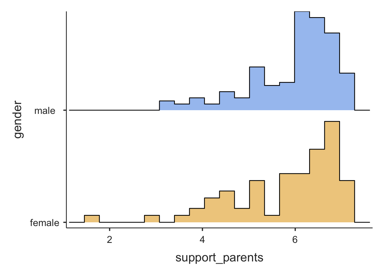
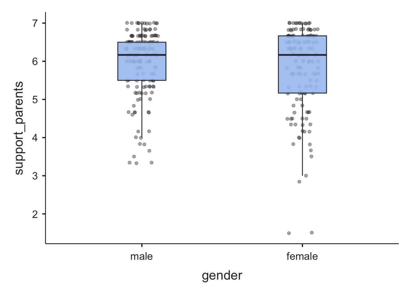
In jamovi (jmv) we use descriptives() again. Let’s look at support_parents and get descriptive statistics (and plots) for male and female adolescents separately:
descriptives(
  formula = support_parents ~ gender,
  data = adolescents,
  hist = TRUE,     # histogram
  box = TRUE,      # box plot
  dot = TRUE,      # add data points to box plot
  median = FALSE,  # Median (deselected here since included in pc below)
  sd = TRUE,       # Standard Deviation
  variance = TRUE, # Variance
  se = TRUE,       # Standard Error of the Mean
  skew = TRUE,     # Skewness
  kurt = TRUE,     # Kurtosis
  pc = TRUE,       # percentiles
  pcValues = "25, 50, 75") # percentile values
##
## DESCRIPTIVES
##
## Descriptives
## ────────────────────────────────────────────────────
## gender support_parents
## ────────────────────────────────────────────────────
## N male 151
## female 134
## Missing male 1
## female 0
## Mean male 5.944150
## female 5.790050
## Std. error mean male 0.07069892
## female 0.09703328
## Standard deviation male 0.8687628
## female 1.123241
## Variance male 0.7547489
## female 1.261671
## Minimum male 3.333333
## female 1.500000
## Maximum male 7.000000
## female 7.000000
## Skewness male -1.204500
## female -1.332349
## Std. error skewness male 0.1973942
## female 0.2092858
## Kurtosis male 1.088983
## female 2.016779
## Std. error kurtosis male 0.3923184
## female 0.4156419
## 25th percentile male 5.500000
## female 5.166667
## 50th percentile male 6.166667
## female 6.166667
## 75th percentile male 6.500000
## female 6.666667
## ────────────────────────────────────────────────────
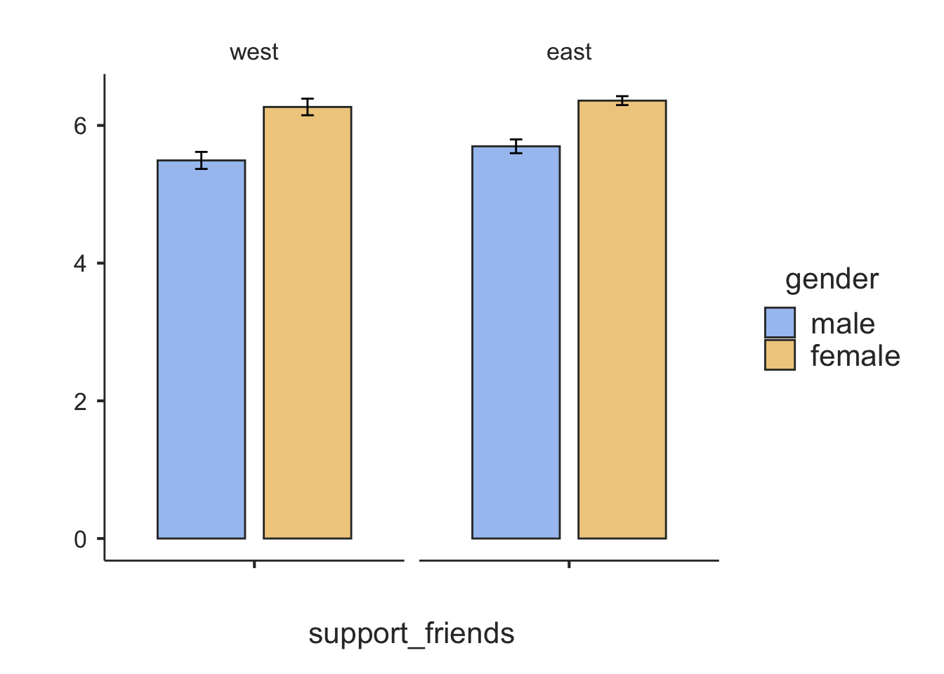
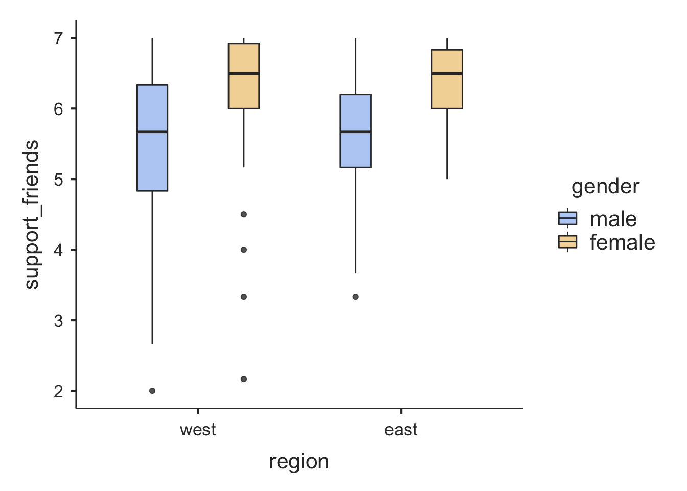
Let’s look at the perceived support from friends (support_friends) for comparison, and add a second factor:
descriptives(
  formula = support_friends ~ gender:region,
  data = adolescents,
  min = FALSE,
  max = FALSE,
  missing = FALSE,
  sd = TRUE,
  bar = TRUE,  # bar plot of means
  box = TRUE)
##
## DESCRIPTIVES
##
## Descriptives
## ─────────────────────────────────────────────────────────────
## gender region support_friends
## ─────────────────────────────────────────────────────────────
## N male west 83
## east 69
## female west 59
## east 74
## Mean male west 5.491767
## east 5.696860
## female west 6.268362
## east 6.360360
## Median male west 5.666667
## east 5.666667
## female west 6.500000
## east 6.500000
## Standard deviation male west 1.126667
## east 0.8313372
## female west 0.9259028
## east 0.5565625
## ─────────────────────────────────────────────────────────────
7.3.3 Descriptive statistics for metric variables using the psych package
install.packages("psych")
The psych package provides some nice functionality for data analysis in psychology. For example, it has a useful function for descriptive statistics for numerical variables: describe(). The generic form is: describe(x, na.rm = TRUE, interp = FALSE, skew = TRUE, ranges = TRUE, trim = 0.1, type = 3, check = TRUE).
x stands for the data frame or the variable to be analyzed (df$variable). The defaults are:
interp = FALSErefers to the definition of the median (interp = TRUEaverages adjacent values for an even n)skew = TRUEdisplays skewness, kurtosis and the trimmed meanranges = TRUEdisplays min, max, the range, the median, and the mad (median average deviation, an alternative measure of dispersion)trim = 0.1refers to the proportion of the distribution that is trimmed at the lower and upper ends for the trimmed mean (default trimming is 10% on both sides, thus the trimmed mean is computed from the middle 80% of the data)type = 3refers to the method of computing skewness and kurtosis (more here:?psych::describe)check = TRUErefers to checking for non-numeric variables in the dataset (for whichdescribehas no use); ifcheck = FALSEand there are non-numeric variables, an error message is displayed.
library(psych)
adolescents %>%
  select(support_parents, support_friends) %>%
  describe()
## vars n mean sd median trimmed mad min max range skew
## support_parents 1 285 5.87 1.00 6.17 6.01 0.74 1.5 7 5.5 -1.35
## support_friends 2 285 5.93 0.96 6.00 6.06 0.99 2.0 7 5.0 -1.25
## kurtosis se
## support_parents 2.05 0.06
## support_friends 1.85 0.06# A somewhat reduced "fast" version
adolescents %>%
select(support_parents, support_friends) %>%
describe(fast = TRUE)## vars n mean sd min max range se
## support_parents 1 285 5.87 1.00 1.5 7 5.5 0.06
## support_friends 2 285 5.93 0.96 2.0 7 5.0 0.067.4 Correlation analysis
7.4.1 Traditional ways of doing correlation analysis in R
The generic form for calculating a correlation matrix using base R is as follows: cor(df[,c("var1", "var2", "var3")], methdod = c("pearson", "kendall", "spearman"), use = "complete.obs").
We can thus compute Pearson correlations (default) or - for ordinal data - Kendall’s \(\tau\) or Spearman’s \(\rho\) rank correlations.
Let’s try it using four scales measuring adolescents’ academic as well as social self-efficacy:
adolescents %>%
    select(se_achievement, se_motivation, se_assertive, se_social) %>%
    cor(method = "pearson", use = "complete.obs") %>%
    round(3)
## se_achievement se_motivation se_assertive se_social
## se_achievement 1.000 0.640 0.351 0.363
## se_motivation 0.640 1.000 0.415 0.407
## se_assertive 0.351 0.415 1.000 0.592
## se_social 0.363 0.407 0.592 1.000For covariances use cov() with the same arguments:
adolescents %>%
    select(se_achievement, se_motivation, se_assertive, se_social) %>%
    cov(method = "pearson", use = "complete.obs") %>%
    round(3)
## se_achievement se_motivation se_assertive se_social
## se_achievement 0.595 0.380 0.266 0.220
## se_motivation 0.380 0.591 0.314 0.246
## se_assertive 0.266 0.314 0.970 0.458
## se_social 0.220 0.246 0.458 0.617A good way to display a scatterplot matrix for a number of variables is the function scatterplotMatrix from the car package.
In addition to displaying all combinations of bivariate scatterplots different univariate plots can be displayed in the diagonal: diagonal = list(method = c("density", "boxplot", "histogram", "oned", "qqplot", "none")). In addition, smooth = TRUE (default) adds a non-linear LOWESS line (LOcally WEighted Scatterplot Smoother) to assess the (non-)linearity of the correlation.
install.packages("car")
library(car)
scatterplotMatrix(~ se_achievement + se_motivation +
                    se_assertive + se_social,
                  smooth = TRUE, # default
                  diagonal = list(method = "histogram"), # if TRUE defaults to "density"
                  data = adolescents,
                  regLine = list(col = "red"), # if omitted defaults to point colour
use = "complete.obs") # default; alternative: "pairwise.complete.obs" 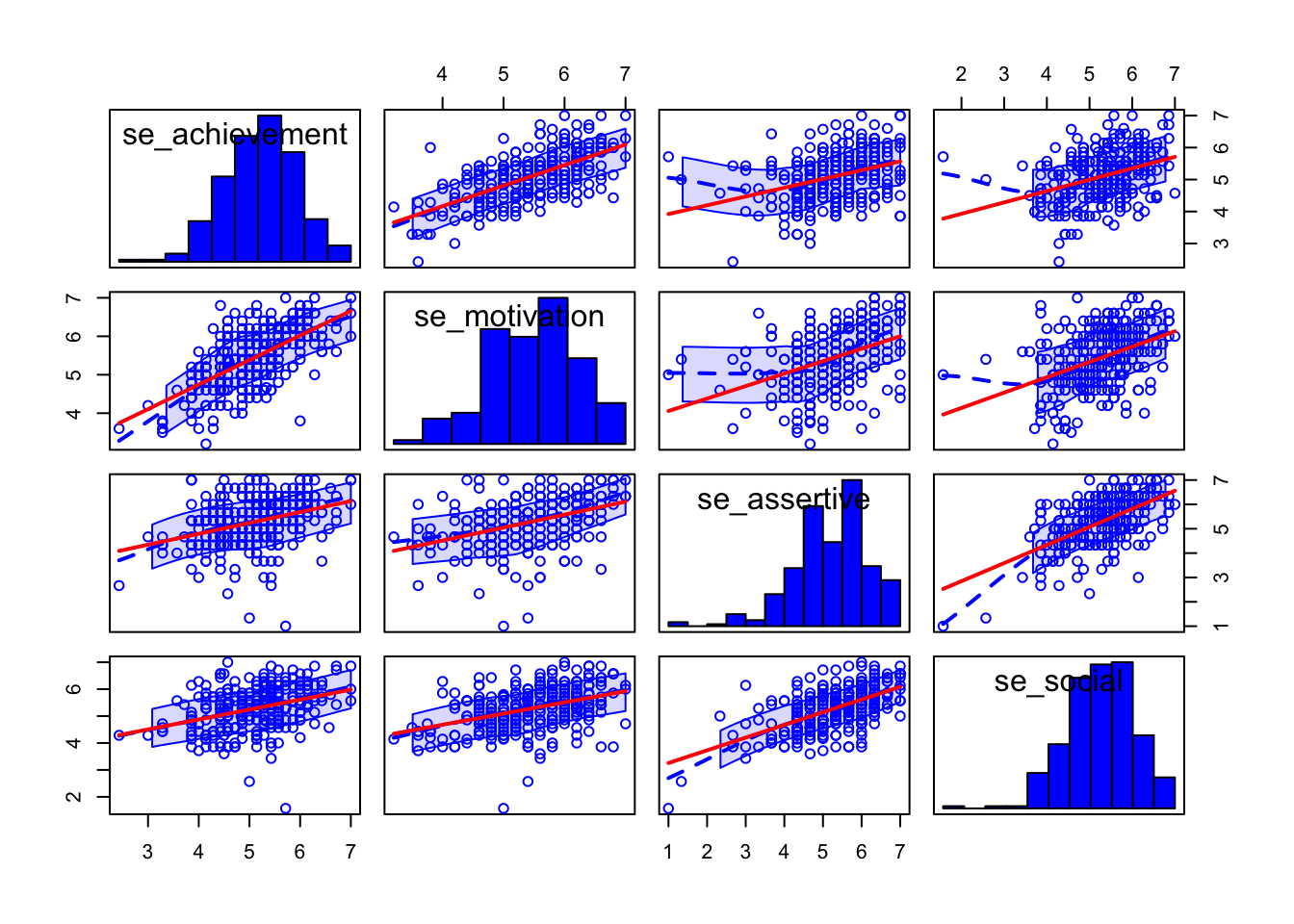
The function cor.test() returns a significance test for one specific correlation.
The generic form is: cor.test (x, y, alternative = c ("two.sided", "less", "greater"), method = c ("pearson", "kendall", "spearman"), conf. level = 0.95).
Thus, in addition to the standard two-sided hypothesis test (alternative = "two.sided"), directional alternative hypotheses are possible: (alternative = "less") for the alternative hypothesis of negative correlation (“less than 0”) and (alternative = "greater") ffor the alternative hypothesis of positive correlation (“greater than 0”).
cor.test(adolescents$se_achievement, adolescents$se_social,
         alternative = "greater",
         method = "pearson")
##
## Pearson's product-moment correlation
##
## data: adolescents$se_achievement and adolescents$se_social
## t = 6.5528, df = 284, p-value = 1.325e-10
## alternative hypothesis: true correlation is greater than 0
## 95 percent confidence interval:
## 0.2746381 1.0000000
## sample estimates:
## cor
## 0.3624033The function corr.test() from the psych package includes \(p\)-values for a correlation matrix. However, no directional alternative hypotheses are possible. Note that the two-sided \(p\)-values are in the lower triangular matrix and the \(p\)-values adjusted according to Holm are in the upper triangular matrix. The Holm procedure corresponds to a sequential alpha correction that is less conservative than the Bonferroni procedure, but nevertheless controls the family-wise error. In the diagonals \(p\)-values for the variances of the variables are displayed.
In the Holm procedure (Bonferroni-Holm method), the smallest \(p\)-value is multiplied by the number of tests (\(p(p-1)/2\); \(p\) = number of variables in the correlation matrix), the second smallest by the number of tests minus 1, etc. until the largest \(p\)-value that is no longer corrected. However, the \(p\)-value is only multiplied by the corresponding number of tests if the resulting adjusted \(p\)-value is not smaller than the previously adjusted (smaller) \(p\)-value. If the latter occurs, the test is assigned the same \(p\)-value as the previous test. This prevents that a smaller effect may reach significance while a larger effect does not.
Let’s try it for the four self-efficacy scales, but use only the first 25 subjects (lines) to make sure we obtain differences between the adjusted and unadjusted \(p\)-values (because with the full sample all correlations are significant beyond \(p<.001\))
library(psych)
adolescents[1:25,] %>%
  select(se_achievement, se_motivation, se_assertive, se_social) %>%
    corr.test()
## Call:corr.test(x = .)
## Correlation matrix
## se_achievement se_motivation se_assertive se_social
## se_achievement 1.00 0.57 0.22 0.19
## se_motivation 0.57 1.00 0.52 0.50
## se_assertive 0.22 0.52 1.00 0.90
## se_social 0.19 0.50 0.90 1.00
## Sample Size
## [1] 25
## Probability values (Entries above the diagonal are adjusted for multiple tests.)
## se_achievement se_motivation se_assertive se_social
## se_achievement 0.00 0.02 0.57 0.57
## se_motivation 0.00 0.00 0.03 0.03
## se_assertive 0.29 0.01 0.00 0.00
## se_social 0.36 0.01 0.00 0.00
##
## To see confidence intervals of the correlations, print with the short=FALSE option7.4.2 Correlation analysis with jmv
Almost all we have done above with the more traditional R functions we can also do in jmv using the corrMatrix() function. An overview of the available arguments is provided by ?jmv::corrMatrix:
corrMatrix(data, vars, pearson = TRUE, spearman = FALSE, kendall = FALSE,
  sig = TRUE, flag = FALSE, ci = FALSE, ciWidth = 95, plots = FALSE,
  plotDens = FALSE, plotStats = FALSE, hypothesis = "corr")

Arguments

data        the data as a data frame
vars          a vector of strings naming the variables to correlate in data
pearson     TRUE (default) or FALSE, provide Pearson's R
spearman    TRUE or FALSE (default), provide Spearman's rho
kendall     TRUE or FALSE (default), provide Kendall's tau-b
sig         TRUE (default) or FALSE, provide significance levels
flag          TRUE or FALSE (default), flag significant correlations
ci          TRUE or FALSE (default), provide confidence intervals
ciWidth     a number between 50 and 99.9 (default: 95), the width of CI
plots         TRUE or FALSE (default), provide a correlation matrix plot
plotDens    TRUE or FALSE (default), provide densities in the correlation matrix plot
plotStats     TRUE or FALSE (default), provide statistics in the correlation matrix plot
hypothesis  one of 'corr' (default), 'pos', 'neg' specifying the alernative hypothesis;
            correlated, correlated positively, correlated negatively respectively.
Correlations of the four self-efficacy variables with one-sided tests (for hypotheses of positive correlations):
library(jmv)
adolescents25 <- adolescents[1:25,]
corrMatrix(
  data = adolescents25,
  vars = vars(se_achievement,
              se_motivation,
              se_assertive,
              se_social),
  n = TRUE,
  hypothesis = "pos")
##
## CORRELATION MATRIX
##
## Correlation Matrix
## ─────────────────────────────────────────────────────────────────────────────────────────────────
## se_achievement se_motivation se_assertive se_social
## ─────────────────────────────────────────────────────────────────────────────────────────────────
## se_achievement Pearson's r —
## p-value —
## N —
##
## se_motivation Pearson's r 0.5680460 —
## p-value 0.0015273 —
## N 25 —
##
## se_assertive Pearson's r 0.2216103 0.5154776 —
## p-value 0.1435212 0.0041791 —
## N 25 25 —
##
## se_social Pearson's r 0.1908148 0.5033212 0.8989274 —
## p-value 0.1804469 0.0051617 < .0000001 —
## N 25 25 25 —
## ─────────────────────────────────────────────────────────────────────────────────────────────────
## Note. Hₐ is positive correlation