2 An introduction to the R language
While R is a general purpose programming language, its main purpose is to provide a specialized programming environment for data analysis, and this is reflected in the language design. R was created by statisticians, for statisticians, and has not seen as widespread an adoption, as for example Python.
As with any language, be it a natural or a programming language, we first need to master
some basic vocabulary. This includes both operators and functions. We will
focus on how to use functions. This is followed by a look at the
fundamental data types, leading us to the most important object for
statistical applications, the data frame. We will look at a modern version
of the data frame, the tibble, which in many ways is an improvement over the
old data frame. We will thus often refer to data frames, even when we are
technically working with tibbles.
2.1 Operators and functions
To start with, let us look at some arithmetic and logical operators. Operators
are generally used between two arguments, like this: 1 + 2. This is known as
infix notation. Function, on the other hand, are applied to their arguments
like so: abs(x). In this case, the function is abs() and its only argument is the data argument x. If x is a real number, abs(x) will return the absolute value of that number.
Operators in R are just special functions, which are allowed
to be used in between two operands. The operator + is actually a function; it
can also be used as a function. In this case, it needs to be surrounded by
backticks
`+`(1, 2)2.1.1 Arithmetic operators
The first five should be self-explanatory:
+                addition
-                subtraction
*                multiplication
/                division
^ or **          power

x %*% y          matrix multiplication c(5, 3) %*% c(2, 4) == 22
x %% y           modulo (x mod y) 5 %% 2 == 1
x %/% y          whole number division: 5 %/% 2 == 2
The last three operators may be new to you.
%*% is the operator for matrix multiplication. %% is the modulo operator. This finds the
remainder after division, e.g. 5 %% 2 (5 modulo 2) is equal to 1. %/% is
used for whole number division, e.g. 5 %/% 2 is equal to 2 (how many times is 2
contained in 5?). These operators are often used for programming.
2.1.2 Logical operators and functions
<                less than
<=               less than or equal to
>                greater than
>=               greater than or equal to
==               equal
!=               not equal
!x               not x (negation)
x | y            x OR y
x & y            x AND y
xor(x, y)        exclusive OR (either in x or y, but not in both)
The following provides a visual overview of the logical operators using Venn diagrams. x refers to the left circle, y to the right circle.
](figures/transform-logical.png)
Figure 2.1: Logical operators. From R for Data Science
2.1.3 Some basic numerical functions
The following is a list of some functions that are used for mathematical
operations. For instance log() computes the natural logarithm of its argument.
We can compute the logarithm to any base using the function’s second argument base.
abs(x)             absolute value
sqrt(x)            square root
ceiling(x)         round up: ceiling(3.475) is 4
floor(x)           round down: floor(3.475) is 3
round(x, digits=n) round: round(3.475, digits=2) is 3.48
log(x)             natural logarithm
log(x, base = n)  base n logarithm
log2(x)            base 2 logarithm
log10(x)           base 10 logarithm
exp(x)             exponential function: e^x
2.1.4 Using R as a calculator
We are ready to do some basic math. Try out the following examples in the R console.
# addition
5 + 5
12321 + 343224

# subtraction
6 - 5
5 - 89

# multiplication
3 * 5
34 * 54

# division
4 / 9
(5 + 5) / 2

# parentheses are important
(3 + 7 + 2 + 8) / (4 + 11 + 3)
1/2 * (12 + 14 + 10)
1/2 * 12 + 14 + 10

# power
3^2
2^12

# exponential function
exp(5)

# the next result is given in scientific notation:
# 1.068647 * 10^13
exp(30)
# whole number division
# 6 is contained 5 times in 33, with remainder 3
33 %% 6 # remainder: 3## [1] 333 %/% 6 # contained 5 times## [1] 55 %% 2 # remainder 1## [1] 15 %/% 2 # contained twice## [1] 2# logical operators
3 > 2## [1] TRUE4 > 5## [1] FALSE4 < 4## [1] FALSE4 <= 4## [1] TRUE6 != 6## [1] FALSE9 == 5 + 4## [1] TRUE!(3 > 2)## [1] FALSE(3 > 2) & (4 > 5) # AND## [1] FALSE(3 > 2) | (4 > 5) # OR## [1] TRUExor((3 > 2), (4 > 5))## [1] TRUE2.1.5 Statistical functions
Here is a list of basic statistical functions. These have in common that they can have
the argument na.rm, which lets us deal with missing values (na stands for not available) and is set to FALSE by default. If set to FALSE, existing nas are not removed before applying the function (rm stands for remove). In this case the function will return itself the value NA because it cannot be applied over nas. Thus, if you want to make sure the function computes the statistic for the available data and thus nas are removed before applying the function (this is what we usually want), make sure to set na.rm = TRUE.
mean(x, na.rm = FALSE)  mean
sd(x)                   standard deviation
var(x)                  variance

median(x)               median
quantile(x, probs)      quantile of x.  probs: vector of probabilities

sum(x)                  sum
min(x)                  minimal value of x (x_min)
max(x)                  maximal value of x (x_max)
range(x)                x_min und x_max

scale(x, center = TRUE, scale = TRUE)   center and standardize
# center = TRUE: subtract mean
# scale = TRUE: divide by sd


sample(x, size, replace = FALSE, prob)  sampling with or without replacement
                                        prob: vector of weights
2.1.6 Further useful functions
One of the most often used functions is c(). This stands for combine or
concatenate; it is used to combine individual elements into a vector.
c()                    combine: used to create a vector
seq(from, to, by)      generates a sequence
:                      colon operator: generates a sequence in increments of 1
rep(x, times, each)    repeats x
                          times: sequence is repeated n times
                          each: each element is repeated n times

head(x, n = 6)         show first 6 elements of x
tail(x, n = 6)         show last 6 elements of x
2.1.7 Examples
# this creates a vector consisting of the elements 1 to 6
c(1, 2, 3, 4, 5, 6)
## [1] 1 2 3 4 5 6mean(c(1, 2, 3, 4, 5, 6))## [1] 3.5mean(c(1, NA, 3, 4, 5, 6), na.rm = TRUE)## [1] 3.8mean(c(1, NA, 3, 4, 5, 6), na.rm = FALSE)## [1] NAsd(c(1, 2, 3, 4, 5, 6))## [1] 1.870829sum(c(1, 2, 3, 4, 5, 6))## [1] 21min(c(1, 2, 3, 4, 5, 6))## [1] 1range(c(1, 2, 3, 4, 5, 6))## [1] 1 6scale(c(1, 2, 3, 4, 5, 6), center = TRUE, scale = FALSE)## [,1]
## [1,] -2.5
## [2,] -1.5
## [3,] -0.5
## [4,] 0.5
## [5,] 1.5
## [6,] 2.5
## attr(,"scaled:center")
## [1] 3.5scale(c(1, 2, 3, 4, 5, 6), center = TRUE, scale = TRUE)## [,1]
## [1,] -1.3363062
## [2,] -0.8017837
## [3,] -0.2672612
## [4,] 0.2672612
## [5,] 0.8017837
## [6,] 1.3363062
## attr(,"scaled:center")
## [1] 3.5
## attr(,"scaled:scale")
## [1] 1.870829# sampling with replacement
sample(c(1, 2, 3, 4, 5, 6), size = 12, replace = TRUE)## [1] 2 2 1 1 1 4 1 6 6 3 3 1# weighted sampling with replacement:
sample(c(1, 2, 3, 4, 5, 6), size = 8, replace = TRUE,
prob = c(0.2, 0.1, 0.05, 0.05, 0.3, 0.3))## [1] 5 5 5 1 1 6 6 1# weighted sampling without replacement:
sample(c(1, 2, 3, 4, 5, 6), size = 3, replace = FALSE,
prob = c(0.2, 0.1, 0.05, 0.05, 0.3, 0.3))## [1] 5 1 6# the following two examples create a sequence from 1 to 6. This gives the same
# result as c(1, 2, 3, 4, 5, 6)
seq(from = 1, to = 6, by = 1)## [1] 1 2 3 4 5 61:6## [1] 1 2 3 4 5 6# the colon operator is often used to create a 'regular' sequence (i.e. a sequence in steps of 1)
# rep() can be used to create special vectors where values and sequences are repeated in a specific manner
rep(1:6, times = 2)## [1] 1 2 3 4 5 6 1 2 3 4 5 6rep(1:6, each = 2)## [1] 1 1 2 2 3 3 4 4 5 5 6 6rep(1:6, times = 2, each = 2)## [1] 1 1 2 2 3 3 4 4 5 5 6 6 1 1 2 2 3 3 4 4 5 5 6 62.2 Defining variables
Variables are usually defined in R using the asssignment arrow <-: my_var <- 4. We have already seen this in examples above when defining a vector.
The assignment operator <- is somewhat tedious to type, a useful shortcut therefore is ALT + -. Interestingly, both <- and = can be used for assignment in R. Purists prefer <-, mainly for historical reasons and because = is then reserved for assigning values to arguments (in functions, e.g., na.rm = TRUE), and thus variable assignment and the selection of values (options) for function arguments do not use the same operator.
Now let us define my_var by assigning the value 4 to it:
my_var <- 4Check the Environment pane. You should see new variables appearing there. A variable with only one value is actually a constant (because there is no variation). It can also be conceived of as a vector with only 1 element, a so-called ‘scalar’.
my_var exists now in the Global Environment, but will no longer be
available when we restart R.
Variable names
A variable needs a name. This must consist of letters, numbers and may contain
_ (underscore) and/or . (period). A name must begin with a letter, and may not contain spaces.
There are a few conventions. We recommend using snake_case for variable names, e.g. my_var.
Other options are:
camelCaseVariable
variable.with.periods
variable.With_noConventions
Many programmers tended to use . in variable names instead of _. Modern style guides do not recommend this, because it can lead to confusion when using S3 object orientation.
2.3 Function calls
Let’s take a closer look at the syntax of R function calls.
The function shown below consists of a name function_name and two arguments,
arg1 and arg2. The arguments may have default values. In this example,
arg1 doesn’t have a default value, but arg2 has the default value val2.
Arguments with no default value are required, whereas arguments with a
default value are not. These simply take their default value if no value is
provided.
function_name(arg1, arg2 = val2)A function may have many arguments.
2.3.1 Nested function calls
Function calls can be nested. This means that the output of one function is passed as input to the next function.
For example: Let’s define a vector, compute its mean and then round to two decimal places:
# define a vector:
c(34.444, 45.853, 21.912, 29.261, 31.558)
## [1] 34.444 45.853 21.912 29.261 31.558# compute mean:
mean(c(34.444, 45.853, 21.912, 29.261, 31.558))## [1] 32.6056# round:
round(mean(c(34.444, 45.853, 21.912, 29.261, 31.558)),
digits = 2)## [1] 32.61Function calls are always performed in the same order: from innermost to outermost, e.g. first c(), then mean() and finally round().
2.4 Data types
Vectors are the fundamental data type in R - all other data types are composed of vectors. These can subdivided into:
numeric vectors: a further subdivision is into
integer(whole numbers) unddouble(double-precision floating point numbers, i.e. the way a computer represents real numbers). For most purposes numeric vectors of thedouble-type are used. Only rarely one has to explicitly defineintegervectors.character vectors: these consist of characters strings and are surrounded by quotes, either single
'or double", e.g.'word'oder"word".logical vectors: these can take three values:
TRUE,FALSEorNA.
Vectors consist of elements of the same type, i.e., we cannot combine logical and character elements in a vector. Vectors have three properties:
- Type:
typeof(): what is it? - Length:
length(): how many elements? - Attribute:
attributes(): additional metadata
Vectors are created using the c() function or by using special function, such as seq() or rep().
2.4.1 Numeric vectors
We have already created numeric vectors above. Let’s do it again!
numbers <- c(1, 2.5, 4.5)
typeof(numbers)
## [1] "double"length(numbers)## [1] 3We can subset vectors, i.e. select individual elements from a vector using []:
# the first element:
numbers[1]
## [1] 1# the second element:
numbers[2]## [1] 2.5# the last element:
# numbers has length 3
length(numbers)## [1] 3# we can use this for subsetting
numbers[length(numbers)]## [1] 4.5# with - (minus) we can omit an element, e.g. the first
numbers[-1]## [1] 2.5 4.5# we can use a sequence
numbers[1:2]## [1] 1.0 2.5# we can omit the first and third elements
numbers[-c(1, 3)]## [1] 2.5Matrices
A matrix is a special kind of vector in R. It is basically a vector that has an additional dim (dimension) attribute:
The following code illustrates how you can create a matrix by changing the
dimensions of a vector, or alternatively by using the matrix() function.
# x is a vector
x <- 1:8

# we can define the dimensions of x
dim(x) <- c(2, 4)
x
## [,1] [,2] [,3] [,4]
## [1,] 1 3 5 7
## [2,] 2 4 6 8# we can also create a matrix like this:
m <- matrix(x <- 1:8, nrow = 2, ncol = 4, byrow = FALSE)
m## [,1] [,2] [,3] [,4]
## [1,] 1 3 5 7
## [2,] 2 4 6 8# what are its dimensions?
dim(m)## [1] 2 4We are using the argument byrow, which has the default value FALSE. If we set this to true (byrow = TRUE) we obtain:
m2 <- matrix(x <- 1:8, nrow = 2, ncol = 4, byrow = TRUE)
m2
## [,1] [,2] [,3] [,4]
## [1,] 1 2 3 4
## [2,] 5 6 7 8With byrow = TRUE the rows are filled in first!
Matrices can be transposed, i.e. the rows become the columns and vice versa:
m_transposed <- t(m)
m_transposed
## [,1] [,2]
## [1,] 1 2
## [2,] 3 4
## [3,] 5 6
## [4,] 7 8There are two further functions that are often used for creating matrices: cbind() and rbind().
cbind() combines several columns vectors to a matrix:
x1 <- 1:3
# x1 is a vector
x1
## [1] 1 2 3x2 <- 10:12
# x2 is a vector
x2## [1] 10 11 12m1 <- cbind(x1, x2)
# m1 is a matrix with dimensions [3, 2]
m1## x1 x2
## [1,] 1 10
## [2,] 2 11
## [3,] 3 12rbind() combines several row vectors to a matrix:
m2 <- rbind(x1, x2)
# m2 is a matrix with dimensions [2, 3]
m2
## [,1] [,2] [,3]
## x1 1 2 3
## x2 10 11 12Just like vectors, matrices can be subset using []. Note that now we need to
specify both rows and columns: [row, column], separated by a comma. If either
row or column is omitted, R selects all rows or columns.
# row 1, column 1
m1[1, 1]
## x1
## 1# row 1, column 2
m1[1, 2]## x2
## 10# rows 2-3, column 1
m1[2:3, 1]## [1] 2 3# all rows, column 1
m1[, 1]## [1] 1 2 3# row 2, all columns
m1[2, ]## x1 x2
## 2 11Vectorization
Everything in R is vectorized, i.e. all functions and operators automatically
operate on whole vectors. E.g. if we create a vector x1 and then add the
number 2 to x1, this is added to each element of x1.
x1 <- 1:10
x1 + 2
## [1] 3 4 5 6 7 8 9 10 11 12x2 <- 11:20
x1 + x2## [1] 12 14 16 18 20 22 24 26 28 30# element-wise multiplication
x1 * x2## [1] 11 24 39 56 75 96 119 144 171 200x1^2## [1] 1 4 9 16 25 36 49 64 81 100Recycling
Something to be aware of is vector recycling: This means that if we perform an
operation with two vectors that don’t have the same length, the shorter vector
is repeated. E.g., if we add two vectors, we get:
# the shorter vector is recycled:
1:10 + 1:2
## [1] 2 4 4 6 6 8 8 10 10 12This is what is happening here:
1  2  3  4  5  6  7  8  9 10
1  2  1  2  1  2  1  2  1  2
The vector 1:2 is repeated as often as necessary.
What happens if the length of the longer vector is not a mupliple of the length of the shorter vector?
1:10 + 1:3## Warning in 1:10 + 1:3: longer object length is not a multiple of shorter object
## length## [1] 2 4 6 5 7 9 8 10 12 11R will give us a warning in this case.
1  2  3  4  5  6  7  8  9 10
1  2  3  1  2  3  1  2  3  1
Missing Values
Missing values are declared with NA.
numbers <- c(12, 13, 15, 11, NA, 10)
numbers
## [1] 12 13 15 11 NA 10We can use the function is.na() to test for missing values:
is.na(numbers)## [1] FALSE FALSE FALSE FALSE TRUE FALSEMissing values are not the same as Inf (infinity) and NaN (not a number).
These occur for instance when you try to divide by zero: 1/0 or 0/0.
A further data type is NULL; this is often used when an argument of a function remains undefined.
1/0 ## [1] Inf0/0 ## [1] NaN2.4.2 Character vectors
Character vectors (strings) are used to represent text. They are defined like numeric vectors except that their elements are set quotation marks:
text <- c("these are", "some", "words")
text
## [1] "these are" "some" "words"typeof(text)## [1] "character"# text has 3 elements:
length(text)## [1] 3letters and LETTERS are special character vectors, so called built-in constants. They contain all (lower-case and upper-case) letters of the English alphabet. Let’s have a look at some subsets of letters (according to their position in the alphabet):
letters[1:3]## [1] "a" "b" "c"letters[10:15]## [1] "j" "k" "l" "m" "n" "o"LETTERS[24:26]## [1] "X" "Y" "Z"A useful function for combining character vectors is paste():
paste(LETTERS[1:3], letters[24:26], sep = "_")## [1] "A_x" "B_y" "C_z"# everything is vectorized!
# special case with sep = "" (i.e. without any separator)
paste0(1:3, letters[5:7])## [1] "1e" "2f" "3g"first_name <- "Ronald Aylmer"
last_name <- "Fisher"
paste("My name is:", first_name, last_name, sep = " ")## [1] "My name is: Ronald Aylmer Fisher"The tidyverse package stringr offers many
useful functions for working with strings. We will see examples of this in later
chapters.
2.4.3 Logical vectors
Logical vectors can take exactly 3 values; TRUE, FALSE or NA.
log_var <- c(TRUE, FALSE, TRUE)
log_var
## [1] TRUE FALSE TRUELogical vectors can be used for indexing (subsetting) other vectors. For example, we might want to extract all elements of a vector that are greater than some value, e.g. all positive numbers.
set.seed(5434) # makes the example reproducible

# draw 10 random numbers from a Gaussian distribution
x <- rnorm(10, mean = 0, sd = 1)
x
## [1] 1.06115528 0.87480990 -0.30032832 1.21965848 0.09860288 1.89862128
## [7] -1.54699798 0.96349219 -0.64968432 -1.09672125# we want all positive numbers:
x > 0## [1] TRUE TRUE FALSE TRUE TRUE TRUE FALSE TRUE FALSE FALSE# we can use this to index x:
x[x > 0]## [1] 1.06115528 0.87480990 1.21965848 0.09860288 1.89862128 0.96349219# we can also save the index
index <- x > 0
# and use this:
x[index]## [1] 1.06115528 0.87480990 1.21965848 0.09860288 1.89862128 0.963492192.4.4 Factors
The numeric, logical, and character vectors we have met so far are atomic vectors, because they are the fundamental data types.
For categorical data, used for grouping, we need a further object type. This is
known as a factor. A factor is simply a vector of integers, with additional
metadata (attributes). These consist of the object class factor and the factor
levels.
# this is a character vector indicating the gender of a sample of people
gender <- c("male", "female", "male", "male",  "diverse", "female")
gender
## [1] "male" "female" "male" "male" "diverse" "female"typeof(gender)## [1] "character"# this has no attributes
attributes(gender)## NULLWe can define a factor:
gender <- factor(gender, levels = c("female", "male", "diverse"))
gender
## [1] male female male male diverse female
## Levels: female male diverse# gender hast type integer
typeof(gender)## [1] "integer"# but `class` factor
class(gender)## [1] "factor"# and attributes levels und class
attributes(gender)## $levels
## [1] "female" "male" "diverse"
##
## $class
## [1] "factor"# levels can be obtained by
levels(gender)## [1] "female" "male" "diverse"If we don’t explicitly define the levels, R uses the labels found in the data and orders them alphabetically for internal representation/definition of levels (this does not affect the order of the data!)
# let's start again with a character vector
gender <- c("male", "female", "male", "male",  "diverse", "female")

# defining a factor without specifying levels can also be done with as.factor()
gender <- factor(gender)
gender <- as.factor(gender)

# now the order of levels is alphabetically
levels(gender)
## [1] "diverse" "female" "male"# order of data is not affected
gender## [1] male female male male diverse female
## Levels: diverse female maleWe can obtain the integer values of a factor by using unclass().
gender## [1] male female male male diverse female
## Levels: diverse female maleunclass(gender)## [1] 3 2 3 3 1 2
## attr(,"levels")
## [1] "diverse" "female" "male"Representing categorical variables as factors is essential for linear models,
and for plotting. For example, if we use dummy coding in a linear model, the
first factor level will automatically be chosen as the reference category. We
can change the ordering using relevel() or (again) factor().
Usingrelevel():
levels(gender)## [1] "diverse" "female" "male"# the result has to be reassigned to the variable
gender <- relevel(gender, ref = "male")
levels(gender)## [1] "male" "diverse" "female"We can also use factor(), but then we need to provide all levels:
gender <- factor(gender, levels = c("male", "diverse", "female"))
gender
## [1] male female male male diverse female
## Levels: male diverse femaleA new way of working with factors: forcats
The above operations can all be performed using the tidyverse package forcats. We will use this package also for more data wrangling later.
Re-levelling a factor can be performed using the function fct_relevel():
library(forcats)
gender <- fct_relevel(gender, "male")
This will change the ordering of the factor levels, so that "male" becomes the
first level. This function has many more options, which are explained in the
function’s help page.
2.4.5 Lists
The next data types are lists. Whereas atomic vectors must be composed of elements of the same type, lists can contain heterogeneous elements (including other lists).
We can define a list using the function list():
x <- list(1:3, "a", c(TRUE, FALSE, TRUE), c(2.3, 5.9))
x
## [[1]]
## [1] 1 2 3
##
## [[2]]
## [1] "a"
##
## [[3]]
## [1] TRUE FALSE TRUE
##
## [[4]]
## [1] 2.3 5.9This list contains a numeric vector, a character, a logical vector and another numeric vector.
# the type of a list is "list"
typeof(x)
## [1] "list"Lists can be indexed just like vectors:
x[1]## [[1]]
## [1] 1 2 3x[2]## [[1]]
## [1] "a"x[3]## [[1]]
## [1] TRUE FALSE TRUEx[4]## [[1]]
## [1] 2.3 5.9Lists can also be indexed using double square brackets, [[. Whereas the single
square bracket [ returns a list containing just that list elements, double
square brackets [[ return the actual contents of the list element. This is
explained very well in R for Data
Science.
x[[1]]## [1] 1 2 3x[[2]]## [1] "a"Lists are very important in R; most statistical functions actually create lists as outputs, and it is useful to know how to deal with these.
Lists can also have named elements:
x <- list(int = 1:3,
          string = "a",
          log = c(TRUE, FALSE, TRUE),
          double = c(2.3, 5.9))
x
## $int
## [1] 1 2 3
##
## $string
## [1] "a"
##
## $log
## [1] TRUE FALSE TRUE
##
## $double
## [1] 2.3 5.9x is a named list. This makes subsetting easier - there is a special operator,
the $ operator, which can be used for selecting named elements of a list. This
can be used together with tab completion. If you type x$ at the R prompt, R
will show all named elements.
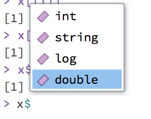
x$string## [1] "a"x$double## [1] 2.3 5.9As an example, the following code performs a two sample t test, and saves the results in a list.
A <- c(1, 1, 3, 4, 2)
B <- c(4, 5, 3, 4, 4.5)
result <- t.test(A, B)
We can inspect the elements of the list. E.g. the p-value can be retrieved like this:
result$p.value ## [1] 0.028118632.4.6 Data frames
We now come to the most important objects for statistics: data frames.
A data frame is a two-dimensional structure with rows and columns. Technically,
a data frame is a list whose elements are equal length vectors. These vectors
can be numeric, logical,character or factors, for categorical (grouping)
variables. A data frame can be subset in the same way as a matrix, or as a list.
A modern version of data frames are referred to as tibbles. tibbles are created using the function tibble().
Let’s create a data frame. We will first use the data.frame() function, and
then create the same data frame using the tibble() function which is provided
by both the dplyr or tibble packages, both of which are automatically loaded
when we load the tidyverse package.
The two main advantages of using tibbles are that (1) strings are never automatically converted into factors (which can lead to problems) and that (2) they have a nicer print method.
df <- data.frame(gender = factor(c("male", "female", "male", "male", "diverse", "female")),
                 age = c(22, 45, 33, 27, 30, 32))
df
## gender age
## 1 male 22
## 2 female 45
## 3 male 33
## 4 male 27
## 5 diverse 30
## 6 female 32library(tidyverse)## ── Attaching packages ─────────────────────────────────────── tidyverse 1.3.1 ──## ✓ ggplot2 3.3.5 ✓ purrr 0.3.4
## ✓ tibble 3.1.5 ✓ dplyr 1.0.7
## ✓ tidyr 1.1.4 ✓ stringr 1.4.0
## ✓ readr 2.0.2## ── Conflicts ────────────────────────────────────────── tidyverse_conflicts() ──
## x dplyr::filter() masks stats::filter()
## x dplyr::lag() masks stats::lag()df <- tibble(gender = factor(c("male", "female", "male", "male", "diverse", "female")),
age = c(22, 45, 33, 27, 30, 32))
df## # A tibble: 6 × 2
## gender age
## <fct> <dbl>
## 1 male 22
## 2 female 45
## 3 male 33
## 4 male 27
## 5 diverse 30
## 6 female 32df is a data frame (or tibble) with two variables, gender and age. This data
frame should appear in the Environment pane (under Data).
A data frame has the attributes names(), colnames() und rownames(); names() und colnames() refer to the same thing.
attributes(df)## $class
## [1] "tbl_df" "tbl" "data.frame"
##
## $row.names
## [1] 1 2 3 4 5 6
##
## $names
## [1] "gender" "age"The length of a data frame is the length of the list, i.e. the number of
colummns. We can also use ncol(). To get the number of rows, we can use
nrow().
ncol(df)## [1] 2nrow(df)## [1] 6Data frame subsetting
Data frames can be subset as a list, or as a matrix.
- as a list: columns (variables) can be selected using
$or[ - as a matrix: elements can be selected using
[
# choose variables
df$gender
## [1] male female male male diverse female
## Levels: diverse female maledf$age## [1] 22 45 33 27 30 32df["gender"]## # A tibble: 6 × 1
## gender
## <fct>
## 1 male
## 2 female
## 3 male
## 4 male
## 5 diverse
## 6 femaledf["age"]## # A tibble: 6 × 1
## age
## <dbl>
## 1 22
## 2 45
## 3 33
## 4 27
## 5 30
## 6 32# by position
df[1]## # A tibble: 6 × 1
## gender
## <fct>
## 1 male
## 2 female
## 3 male
## 4 male
## 5 diverse
## 6 femaledf[2]## # A tibble: 6 × 1
## age
## <dbl>
## 1 22
## 2 45
## 3 33
## 4 27
## 5 30
## 6 32We can also select rows and columns, just as we would do with a matrix: [row, column].
# row 1, column 1
df[1, 1]
## # A tibble: 1 × 1
## gender
## <fct>
## 1 male# row 1, all columns
df[1, ]## # A tibble: 1 × 2
## gender age
## <fct> <dbl>
## 1 male 22# all rows, column 1
df[, 1]## # A tibble: 6 × 1
## gender
## <fct>
## 1 male
## 2 female
## 3 male
## 4 male
## 5 diverse
## 6 female# all rows, all columns
df[ , ]## # A tibble: 6 × 2
## gender age
## <fct> <dbl>
## 1 male 22
## 2 female 45
## 3 male 33
## 4 male 27
## 5 diverse 30
## 6 female 32# first 3 rows, all columns
df[1:3, ]## # A tibble: 3 × 2
## gender age
## <fct> <dbl>
## 1 male 22
## 2 female 45
## 3 male 33We can also index individual columns (variables):
df$gender[1]## [1] male
## Levels: diverse female male