10 CFA and SEM with lavaan
10.1 Confirmatory Factor Analysis (CFA)
Lavaan is a free open source package for latent variable modeling in R. The lavaan package is developed and maintained by Yves Rosseel (Rosseel, 2012; see also http://lavaan.ugent.be). The name lavaan refers to latent variable analysis. Lavaan can be used to estimate a variety of statistical models: path analysis, structural equation models (SEM) and confirmatory factor analyses (CFA).
10.1.1 Setup: Packages and data
pacman::p_load(tidyverse, ggplot2, ggthemes, haven, lavaan, lavaanPlot, knitr, psych,
               semPlot, semTools, wesanderson)
# Import data
data <- read_sav("data/adolescents_ls.sav")
# Select life satisfaction items
ls <- data %>%
select(num_range("life", 1:10)) %>%
drop_naThe life satisfaction data consist of 10 items relating to different aspects/areas of life satisfaction. The adolescents were asked:
“How satisfied are you with…?”
| Items | |
|---|---|
| life1 | your school grade |
| life2 | your looks and appearance |
| life3 | your relationship with your teacher |
| life4 | your school life |
| life5 | your social life |
| life6 | your personality |
| life7 | your relationships with your friends |
| life8 | your relationship with your parents |
| life9 | your family life |
| life10 | your socio-economic status |
The response was on a 7-point scale from 1 = “not satisfied at all” to 7 = “very satisfied”.
The questions on life satisfaction can be divided into four domains. We rename the variables in such a way that it becomes clear which LS domain they belong to. To bring the order of the variables in line with their content domains, we also change the order using select().
ls <- ls %>%
  rename(fam1 = life8,
         fam2 = life9,
         fam3 = life10,
         school1 = life1,
         school2 = life3,
         school3 = life4,
         self1 = life2,
         self2 = life6,
         friends1 = life5,
         friends2 = life7
         ) %>%
  select(school1, school2, school3, self1, self2,
         friends1, friends2, fam1, fam2, fam3)
Remove outliers
The ML estimation assumes a multivariate normal distribution. We can check multivariate skewness and kurtosis (Mardia’s coefficients):
mardiaSkew(ls, use = "everything")
#>           b1d           chi            df             p
#>  3.209181e+01  1.476223e+03  2.200000e+02 9.489595e-185
mardiaKurtosis(ls, use = "everything")
#>       b2d         z         p
#> 191.24697  38.20193   0.00000
Both skewness and kurtosis are very high, pointing to multivariate outliers that might inflate standard errors of coefficients (coefficients themselves are mostly unaffected by non-normality).
Thus, we remove all subjects/observations with values outside +/- 3 SD from the mean on at least one of the ten life satisfaction variables. By removing univariate outliers we also want to make sure that influential data points play no role for the factor solution.
# Definition of a `keep` function that only selects data points that are between
# +/- 3 standard deviations of a variable
keep <- function(x) {
(x >= mean(x) - 3*sd(x)) &
(x <= mean(x) + 3*sd(x))
}
# Selecting these data points with `filter` and assigning them to a new data set
ls_clean <- ls %>%
  filter(keep(school1) &
           keep(school2) &
           keep(school3) &
           keep(self1) &
           keep(self2) &
           keep(friends1) &
           keep(friends2) &
           keep(fam1) &
           keep(fam2) &
           keep(fam3))
Check Mardia’s coefficients again:
mardiaSkew(ls_clean, use = "everything")
#>          b1d          chi           df            p
#> 1.306214e+01 5.551409e+02 2.200000e+02 6.851861e-31
mardiaKurtosis(ls_clean, use = "everything")
#>          b2d            z            p
#> 1.370003e+02 8.761739e+00 1.922612e-18
Much smaller but still significant!
10.1.2 Defining the CFA model in lavaan
The calculation of a CFA with lavaan in done in two steps: in the first step, a model defining the hypothesized factor structure has to be set up; in the second step this model is estimated using cfa(). This function takes as input the data as well as the model definition. Model definitions in lavaan all follow the same type of syntax.
In the syntax, certain characters (operators) are predefined and a number of default settings are applied. For example, by default the scaling of the latent variable is achieved by fixing the loading of the first indicator (manifest variable) for a certain latent variable to the value of 1.
=~ means that the latent variable (here named Factor1) to the left of the operator is defined by all variables to the right of it. The manifest (measured) variables from the dataset on the right are separated by a +.
An example of six items explained by two factors (latent variables):
example_model <- "
Factor1 =~ var1 + var2 + var3
Factor2 =~ var4 + var5 + var6
# The order of the manifest variables is relevant only for fixing one loading per factor.
# Here the loadings of `var1` and `var4` are set to the value 1.

# Comments like this are ignored by lavaan.
"
The parameters of the model do not have to be explicitly defined (e.g. l12 for the loading of the second item (var2) on the first factor (Factor1). However, they could be defined explicitly and we will see below that this is necessary in some situations.
Another default is that factor variances and covariances are automatically specified for all latent variables in a CFA. The operator for specifying a variance/covariance is ~~. Variances are defined as covariances of a variable with itself. I.e. in this example we could add the lines Factor1 ~~ Factor1, Factor2 ~~ Factor2 (latent variable variances), and Factor1 ~~ Factor2 (latent variable covariance) without changing the model definition. The same holds for the residual variances of the manifest variables (but not for potential residual covariances!).
10.1.3 Estimating the model
Syntax for estimation: cfa(model = example_model, data = dataframe)
However, the direct execution of this syntax results in only a very limited output, containing only the number of estimated parameters, the number of observations, and the chi-square statistics.
Therefore, the result of cfa() must first be assigned to an output object (e.g. fit_example_model) and the detailed output (including the parameter estimates) extracted with summary(fit_example_model). For the summary()-function there are some additional arguments: fit.measures = TRUE outputs a number of global fit indices (e.g. SRMR, RMSEA, CLI, TLI) as well as information criteria (e.g. AIC and BIC), and with standardized = TRUE we get the standardized parameter estimators as well as the unstandardized parameter estimators.
10.1.4 CFA with four factors
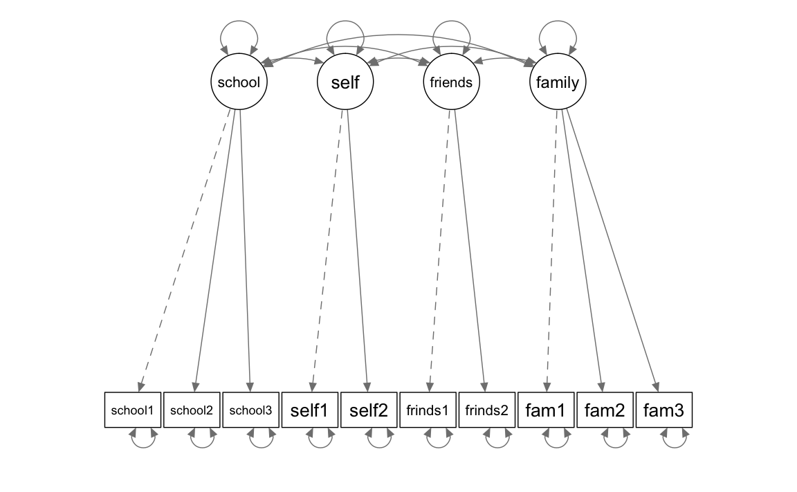
For theoretical reasons, we first estimate a model with four factors. We define one factor for each content domain of life satisfaction (school, self, friends, family). In addition, as usual we postulate a simple structure, i.e. all potential cross-loadings are restricted to the value 0 (manifest variables appear only in the equation of their respective factor).
Modell definition
model_4f <- "
school =~ school1 + school2 + school3
self =~ self1 + self2
friends =~ friends1 + friends2
family =~ fam1 + fam2 + fam3
"
In a figure:
Model estimation
fit_mod4f <- cfa(model_4f, data = ls_clean)
summary(fit_mod4f, fit.measures = TRUE, standardized = TRUE)
#> lavaan 0.6-4 ended normally after 40 iterations
#>
#>   Optimization method                           NLMINB
#>   Number of free parameters                         26
#>
#>   Number of observations                           255
#>
#>   Estimator                                         ML
#>   Model Fit Test Statistic                      51.433
#>   Degrees of freedom                                29
#>   P-value (Chi-square)                           0.006
#>
#> Model test baseline model:
#>
#>   Minimum Function Test Statistic              583.039
#>   Degrees of freedom                                45
#>   P-value                                        0.000
#>
#> User model versus baseline model:
#>
#>   Comparative Fit Index (CFI)                    0.958
#>   Tucker-Lewis Index (TLI)                       0.935
#>
#> Loglikelihood and Information Criteria:
#>
#>   Loglikelihood user model (H0)              -3427.760
#>   Loglikelihood unrestricted model (H1)      -3402.044
#>
#>   Number of free parameters                         26
#>   Akaike (AIC)                                6907.520
#>   Bayesian (BIC)                              6999.593
#>   Sample-size adjusted Bayesian (BIC)         6917.166
#>
#> Root Mean Square Error of Approximation:
#>
#>   RMSEA                                          0.055
#>   90 Percent Confidence Interval          0.029  0.079
#>   P-value RMSEA <= 0.05                          0.341
#>
#> Standardized Root Mean Square Residual:
#>
#>   SRMR                                           0.053
#>
#> Parameter Estimates:
#>
#>   Information                                 Expected
#>   Information saturated (h1) model          Structured
#>   Standard Errors                             Standard
#>
#> Latent Variables:
#>                    Estimate  Std.Err  z-value  P(>|z|)   Std.lv  Std.all
#>   school =~
#>     school1           1.000                               0.572    0.420
#>     school2           1.431    0.257    5.572    0.000    0.819    0.638
#>     school3           1.995    0.403    4.947    0.000    1.141    0.858
#>   self =~
#>     self1             1.000                               0.730    0.669
#>     self2             0.940    0.156    6.028    0.000    0.685    0.784
#>   friends =~
#>     friends1          1.000                               0.661    0.791
#>     friends2          0.614    0.117    5.235    0.000    0.406    0.531
#>   family =~
#>     fam1              1.000                               0.782    0.742
#>     fam2              1.061    0.129    8.233    0.000    0.830    0.846
#>     fam3              0.598    0.084    7.136    0.000    0.467    0.510
#>
#> Covariances:
#>                    Estimate  Std.Err  z-value  P(>|z|)   Std.lv  Std.all
#>   school ~~
#>     self              0.075    0.039    1.947    0.052    0.180    0.180
#>     friends           0.111    0.039    2.862    0.004    0.293    0.293
#>     family            0.098    0.040    2.427    0.015    0.219    0.219
#>   self ~~
#>     friends           0.296    0.059    5.049    0.000    0.614    0.614
#>     family            0.142    0.052    2.735    0.006    0.249    0.249
#>   friends ~~
#>     family            0.178    0.048    3.700    0.000    0.344    0.344
#>
#> Variances:
#>                    Estimate  Std.Err  z-value  P(>|z|)   Std.lv  Std.all
#>    .school1           1.528    0.147   10.414    0.000    1.528    0.824
#>    .school2           0.978    0.137    7.130    0.000    0.978    0.593
#>    .school3           0.469    0.209    2.245    0.025    0.469    0.265
#>    .self1             0.656    0.100    6.575    0.000    0.656    0.552
#>    .self2             0.295    0.076    3.865    0.000    0.295    0.386
#>    .friends1          0.262    0.079    3.301    0.001    0.262    0.375
#>    .friends2          0.419    0.047    8.948    0.000    0.419    0.718
#>    .fam1              0.498    0.079    6.336    0.000    0.498    0.449
#>    .fam2              0.274    0.077    3.574    0.000    0.274    0.285
#>    .fam3              0.622    0.061   10.240    0.000    0.622    0.740
#>     school            0.327    0.109    3.001    0.003    1.000    1.000
#>     self              0.532    0.120    4.452    0.000    1.000    1.000
#>     friends           0.437    0.095    4.594    0.000    1.000    1.000
#>     family            0.611    0.109    5.593    0.000    1.000    1.000
Visualizing the model
We visualize structural equation models using semPlot.
semPaths(fit_mod4f, "par", weighted = FALSE, nCharNodes = 7, shapeMan = "rectangle",
         sizeMan = 8, sizeMan2 = 5)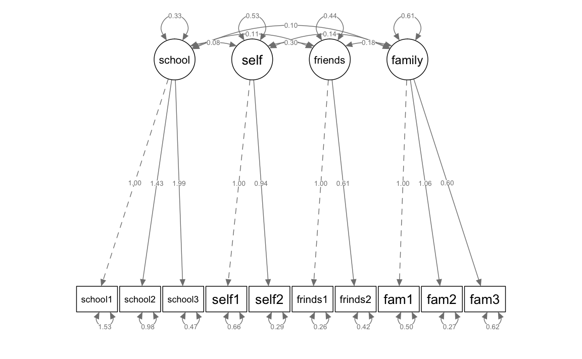
Local model fit: Comparing the empirical and implied variance-covariance matrix
The lavInspect() function allows extracting information from a lavaan object. The argument what specifies which information should be extracted. The value sampstat of this argument stands for “sample statistics”, the empirical variance-covariance matrix:
lavInspect(fit_mod4f, what = "sampstat")
#> $cov
#>          schol1 schol2 schol3 self1 self2 frnds1 frnds2 fam1  fam2  fam3
#> school1  1.855
#> school2  0.444  1.648
#> school3  0.640  0.944  1.771
#> self1    0.104  0.156  0.235  1.189
#> self2    0.167  0.015  0.105  0.500 0.765
#> friends1 0.193  0.088  0.249  0.312 0.271 0.699
#> friends2 0.043  0.095  0.098  0.151 0.183 0.268  0.584
#> fam1     0.369  0.134  0.159  0.136 0.189 0.170  0.168  1.110
#> fam2     0.258  0.162  0.137  0.067 0.118 0.164  0.116  0.656 0.962
#> fam3     0.136  0.173  0.242  0.144 0.198 0.160  0.099  0.326 0.394 0.841
The variance-covariance matrix implied by the model is obtained with what = 'implied':
lavInspect(fit_mod4f, what = "implied")
#> $cov
#>          schol1 schol2 schol3 self1 self2 frnds1 frnds2 fam1  fam2  fam3
#> school1  1.855
#> school2  0.468  1.648
#> school3  0.653  0.934  1.771
#> self1    0.075  0.108  0.150  1.189
#> self2    0.071  0.101  0.141  0.500 0.765
#> friends1 0.111  0.159  0.221  0.296 0.278 0.699
#> friends2 0.068  0.097  0.136  0.182 0.171 0.268  0.584
#> fam1     0.098  0.140  0.196  0.142 0.134 0.178  0.109  1.110
#> fam2     0.104  0.149  0.208  0.151 0.142 0.189  0.116  0.649 0.962
#> fam3     0.059  0.084  0.117  0.085 0.080 0.106  0.065  0.365 0.388 0.841
The smaller the differences between these two matrices, the better the model fits the data, i.e. the closer the variances and covariances recalculated from the estimated parameters are to the empirical variances and covariances.
The residual matrix results from the subtraction of the variance-covariance matrix implied by the model from the observed (empirical) variance-covariance matrix.
residual_matrix <-
  lavInspect(fit_mod4f, what = "sampstat")$cov -
  lavInspect(fit_mod4f, what = "implied")$cov

residual_matrix
#>          schol1 schol2 schol3 self1  self2  frnds1 frnds2 fam1   fam2
#> school1   0.000
#> school2  -0.024  0.000
#> school3  -0.013  0.009  0.000
#> self1     0.028  0.049  0.085  0.000
#> self2     0.096 -0.086 -0.036  0.000  0.000
#> friends1  0.082 -0.070  0.028  0.016 -0.007  0.000
#> friends2 -0.025 -0.002 -0.038 -0.031  0.012  0.000  0.000
#> fam1      0.271 -0.007 -0.037 -0.006  0.055 -0.008  0.059  0.000
#> fam2      0.154  0.013 -0.071 -0.084 -0.023 -0.024  0.001  0.007  0.000
#> fam3      0.077  0.089  0.125  0.059  0.118  0.054  0.034 -0.040  0.006
#>          fam3
#> school1
#> school2
#> school3
#> self1
#> self2
#> friends1
#> friends2
#> fam1
#> fam2
#> fam3      0.000
A direct extraction of the residual matrix is possible with the argument what = "resid":
lavInspect(fit_mod4f, what = "resid")
#> $cov
#>          schol1 schol2 schol3 self1  self2  frnds1 frnds2 fam1   fam2
#> school1   0.000
#> school2  -0.024  0.000
#> school3  -0.013  0.009  0.000
#> self1     0.028  0.049  0.085  0.000
#> self2     0.096 -0.086 -0.036  0.000  0.000
#> friends1  0.082 -0.070  0.028  0.016 -0.007  0.000
#> friends2 -0.025 -0.002 -0.038 -0.031  0.012  0.000  0.000
#> fam1      0.271 -0.007 -0.037 -0.006  0.055 -0.008  0.059  0.000
#> fam2      0.154  0.013 -0.071 -0.084 -0.023 -0.024  0.001  0.007  0.000
#> fam3      0.077  0.089  0.125  0.059  0.118  0.054  0.034 -0.040  0.006
#>          fam3
#> school1
#> school2
#> school3
#> self1
#> self2
#> friends1
#> friends2
#> fam1
#> fam2
#> fam3      0.000
Particularly relevant for the local fit diagnostics is the variance-covariance matrix of standardized residuals. This cannot be obtained using lavInspect(), but with the function resid().
resid(fit_mod4f, type = "standardized")
#> $type
#> [1] "standardized"
#>
#> $cov
#>          schol1 schol2 schol3 self1  self2  frnds1 frnds2 fam1   fam2
#> school1   0.000
#> school2  -0.640  0.000
#> school3  -1.035  2.314  0.000
#> self1     0.336  0.698  1.529  0.000
#> self2     1.437 -1.738 -1.196  0.000  0.000
#> friends1  1.331 -1.659  1.254  1.235 -0.901  0.000
#> friends2 -0.421 -0.044 -0.843 -1.100  0.680  0.000  0.000
#> fam1      3.298 -0.106 -0.764 -0.126  1.645 -0.266  1.560  0.000
#> fam2      2.081  0.243 -2.382 -2.080 -1.010 -1.338  0.017  2.679  0.000
#> fam3      1.064  1.357  1.960  1.080  2.829  1.386  0.892 -2.809  0.790
#>          fam3
#> school1
#> school2
#> school3
#> self1
#> self2
#> friends1
#> friends2
#> fam1
#> fam2
#> fam3      0.000
The following standardisized residuals turn out to be significant (absolute value \(\geq 2.58\: \widehat=\: p\leq 0.01\))
fam1 ~~ schule1 = 3.298
fam3 ~~ selbst2 = -2.829
fam3 ~~ fam1 = -2.809
fam2 ~~ fam1 = 2.679
Global model fit
For CFI = 0.958 and NNFI/TLI = 0.935 values around the recommended cut-off criterion of 0.97/0.95 resulted. The RMSEA = 0.055 is slightly above the cut-off of 0.05, but it is not significantly higher than 0.05 (90 % CI = [0.029; 0.079]). Furthermore, the SRMR = 0.053 points to a good model fit (SRMR < 0.08).
Exemplary computation of CFI, NNFI/TLI, AIC, and BIC:
\(CFI=1-\frac{\chi_{t}^{2}-d f_{t}}{\chi_{i}^{2}-d f_{i}}=1-\frac{51.433-29}{583.039 -45}=1-\frac{22.433}{538.039}=0.958\)
\(NNFI/TLI = \left(\frac{\chi_{i}^{2}}{d f_{i}}-\frac{\chi_{t}^{2}}{d f_{t}}\right)/\left({\frac{\chi_{i}^{2}}{d f_{i}}-1}\right) = \left(\frac{583.039}{45}-\frac{51.433}{29}\right)/\left({\frac{583.039}{45}-1}\right) = \frac{12.956-1.774}{12.956-1} = 0.935\)
\(AIC=-2(logL) + 2 \cdot t= -2 \cdot (-3427.76) + 2 \cdot 26 = 6907.52\)
\(BIC=-2(logL) + \log (n) \cdot t =-2 \cdot (-3427.76) + \log (255) \cdot 26= 6999.59\)
10.1.5 CFA with three factors
Model definition
Since a prior PCA suggested that 3 factors might be enough we want to check this using a CFA approach. Thus, we define an additional model with only three factors (friends and self factors are combined). (Ideally, the PCA should not have been carried out on the same data.)
model_3f <- "
school =~ school1 + school2 + school3
self_friends =~ self1 + self2 + friends1 + friends2
family =~ fam1 + fam2 + fam3
"
Model estimation
fit_mod3f <- cfa(model_3f, data = ls_clean)
summary(fit_mod3f, fit.measures = TRUE, standardized = TRUE)
#> lavaan 0.6-4 ended normally after 39 iterations
#>
#>   Optimization method                           NLMINB
#>   Number of free parameters                         23
#>
#>   Number of observations                           255
#>
#>   Estimator                                         ML
#>   Model Fit Test Statistic                      79.522
#>   Degrees of freedom                                32
#>   P-value (Chi-square)                           0.000
#>
#> Model test baseline model:
#>
#>   Minimum Function Test Statistic              583.039
#>   Degrees of freedom                                45
#>   P-value                                        0.000
#>
#> User model versus baseline model:
#>
#>   Comparative Fit Index (CFI)                    0.912
#>   Tucker-Lewis Index (TLI)                       0.876
#>
#> Loglikelihood and Information Criteria:
#>
#>   Loglikelihood user model (H0)              -3441.804
#>   Loglikelihood unrestricted model (H1)      -3402.044
#>
#>   Number of free parameters                         23
#>   Akaike (AIC)                                6929.609
#>   Bayesian (BIC)                              7011.058
#>   Sample-size adjusted Bayesian (BIC)         6938.142
#>
#> Root Mean Square Error of Approximation:
#>
#>   RMSEA                                          0.076
#>   90 Percent Confidence Interval          0.055  0.098
#>   P-value RMSEA <= 0.05                          0.021
#>
#> Standardized Root Mean Square Residual:
#>
#>   SRMR                                           0.064
#>
#> Parameter Estimates:
#>
#>   Information                                 Expected
#>   Information saturated (h1) model          Structured
#>   Standard Errors                             Standard
#>
#> Latent Variables:
#>                    Estimate  Std.Err  z-value  P(>|z|)   Std.lv  Std.all
#>   school =~
#>     school1           1.000                               0.577    0.424
#>     school2           1.436    0.258    5.574    0.000    0.828    0.645
#>     school3           1.954    0.393    4.971    0.000    1.127    0.847
#>   self_friends =~
#>     self1             1.000                               0.686    0.629
#>     self2             0.889    0.127    7.006    0.000    0.610    0.698
#>     friends1          0.741    0.110    6.722    0.000    0.509    0.608
#>     friends2          0.502    0.092    5.465    0.000    0.344    0.450
#>   family =~
#>     fam1              1.000                               0.787    0.747
#>     fam2              1.048    0.128    8.191    0.000    0.824    0.840
#>     fam3              0.596    0.084    7.131    0.000    0.469    0.511
#>
#> Covariances:
#>                    Estimate  Std.Err  z-value  P(>|z|)   Std.lv  Std.all
#>   school ~~
#>     self_friends      0.103    0.039    2.616    0.009    0.261    0.261
#>     family            0.102    0.041    2.468    0.014    0.225    0.225
#>   self_friends ~~
#>     family            0.178    0.051    3.507    0.000    0.331    0.331
#>
#> Variances:
#>                    Estimate  Std.Err  z-value  P(>|z|)   Std.lv  Std.all
#>    .school1           1.522    0.147   10.379    0.000    1.522    0.821
#>    .school2           0.962    0.139    6.926    0.000    0.962    0.584
#>    .school3           0.501    0.206    2.429    0.015    0.501    0.283
#>    .self1             0.718    0.087    8.236    0.000    0.718    0.604
#>    .self2             0.393    0.057    6.907    0.000    0.393    0.513
#>    .friends1          0.441    0.051    8.572    0.000    0.441    0.630
#>    .friends2          0.466    0.046   10.154    0.000    0.466    0.797
#>    .fam1              0.491    0.079    6.189    0.000    0.491    0.443
#>    .fam2              0.283    0.077    3.700    0.000    0.283    0.295
#>    .fam3              0.621    0.061   10.222    0.000    0.621    0.739
#>     school            0.333    0.110    3.019    0.003    1.000    1.000
#>     self_friends      0.470    0.103    4.571    0.000    1.000    1.000
#>     family            0.619    0.110    5.607    0.000    1.000    1.000
Visualizing the model
semPaths(fit_mod3f, "par", weighted = FALSE, nCharNodes = 7, shapeMan = "rectangle",
         sizeMan = 8, sizeMan2 = 5)
And now with standardized parameter estimates:
semPaths(fit_mod3f, "std", weighted = FALSE, nCharNodes = 7, shapeMan = "rectangle",
         sizeMan = 8, sizeMan2 = 5)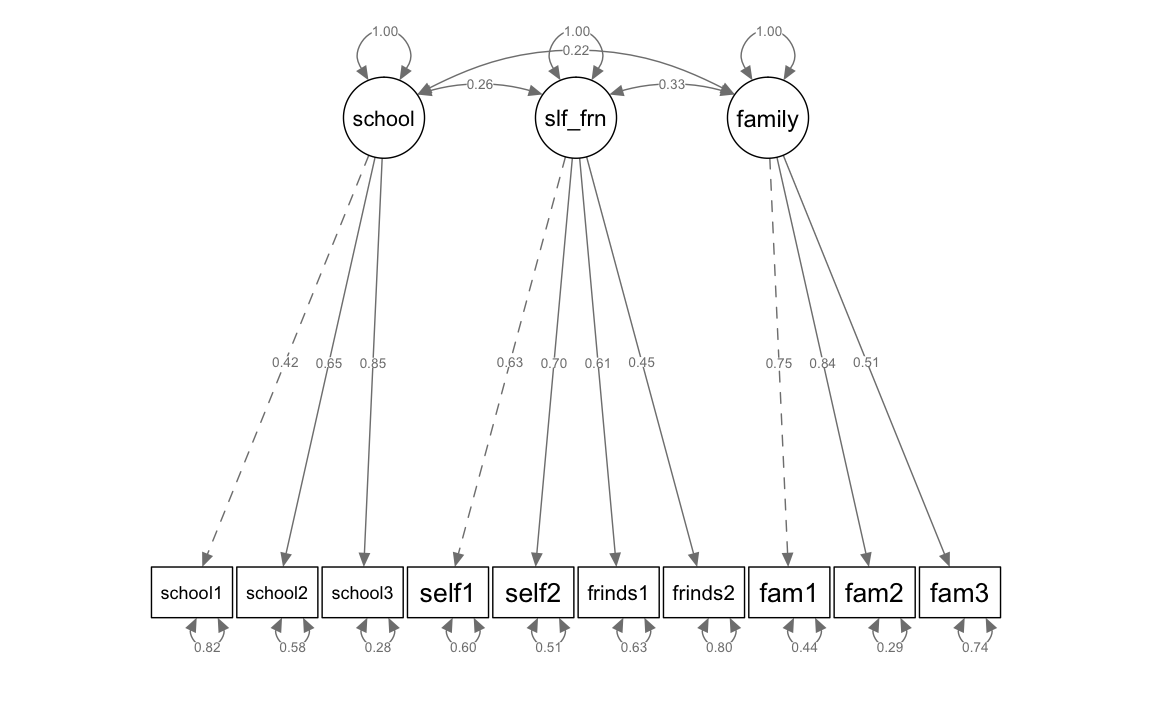
Global model fit
CFI = 0.912 and NNFI/TLI = 0.876 do not reach the recommended cut-off criteria. The RMSEA = 0.076 now is also significantly higher than 0.05 (90 %-CI [0.055; 0.098]).
Alternative definition of the 3-factor model
A 3-factor model can alternatively be specified by restricting certain parameters of the 4-factor model. This allows us to show that the 3-factor model is nested in the 4-factor model.
To turn the 4-factor model into a 3-factor model with a combined self-and-friends-factor, we have to make sure that the factors friends and self behave like a single factor using parameter restrictions.
For these two factors to become one, the covariance between the two factors must be set to 1 (see syntax below). For a covariance of 1 to really represent an exact equality of the two factors, the variances of the two latent variables must also be set to 1 (thus the correlation between the latent variables becomes 1). The easiest way to achieve this is to set the variances of all latent variables to the value 1 using the cfa() argument std.lv = TRUE, which at the same time ensures that the loadings of the first manifest variables of each factor are also estimated freely. This aspect is not defined in the model definition, but in the model estimation.
On the other hand, the relationships of the factors with all other factors must be identical for both factors (friends and self). We can achieve this by naming (i.e. explicitly specifying) the parameters of the factor covariances and at the same time giving the same name to the two parameters to be equated. For example, the covariance of friends and school should be estimated exactly the same as the covariance between self and school. If we name both parameters to be estimated with a, lavaan recognizes that the same value should be estimated for both covariances.
We call this model model_4f_res.
model_4f_res <- "
school =~ school1 + school2 + school3
self =~ self1 + self2
friends =~ friends1 + friends2
family =~ fam1 + fam2 + fam3

# Fixing the covariance to 1
friends ~~ 1*self

# Equality constraints: Covariances with equal parameter names
friends ~~ a*school
self ~~ a*school
friends ~~ b*family
self ~~ b*family
"
Estimating the alternative 3-factor model:
fit_mod4f_res <- cfa(model_4f_res, std.lv = TRUE, data = ls_clean)
summary(fit_mod4f_res, fit.measures = TRUE, standardized = TRUE)
#> lavaan 0.6-4 ended normally after 26 iterations
#>
#>   Optimization method                           NLMINB
#>   Number of free parameters                         25
#>   Number of equality constraints                     2
#>   Row rank of the constraints matrix                 2
#>
#>   Number of observations                           255
#>
#>   Estimator                                         ML
#>   Model Fit Test Statistic                      79.522
#>   Degrees of freedom                                32
#>   P-value (Chi-square)                           0.000
#>
#> Model test baseline model:
#>
#>   Minimum Function Test Statistic              583.039
#>   Degrees of freedom                                45
#>   P-value                                        0.000
#>
#> User model versus baseline model:
#>
#>   Comparative Fit Index (CFI)                    0.912
#>   Tucker-Lewis Index (TLI)                       0.876
#>
#> Loglikelihood and Information Criteria:
#>
#>   Loglikelihood user model (H0)              -3441.804
#>   Loglikelihood unrestricted model (H1)      -3402.044
#>
#>   Number of free parameters                         23
#>   Akaike (AIC)                                6929.609
#>   Bayesian (BIC)                              7011.058
#>   Sample-size adjusted Bayesian (BIC)         6938.142
#>
#> Root Mean Square Error of Approximation:
#>
#>   RMSEA                                          0.076
#>   90 Percent Confidence Interval          0.055  0.098
#>   P-value RMSEA <= 0.05                          0.021
#>
#> Standardized Root Mean Square Residual:
#>
#>   SRMR                                           0.064
#>
#> Parameter Estimates:
#>
#>   Information                                 Expected
#>   Information saturated (h1) model          Structured
#>   Standard Errors                             Standard
#>
#> Latent Variables:
#>                    Estimate  Std.Err  z-value  P(>|z|)   Std.lv  Std.all
#>   school =~
#>     school1           0.577    0.096    6.037    0.000    0.577    0.424
#>     school2           0.828    0.097    8.499    0.000    0.828    0.645
#>     school3           1.127    0.111   10.109    0.000    1.127    0.847
#>   self =~
#>     self1             0.686    0.075    9.141    0.000    0.686    0.629
#>     self2             0.610    0.060   10.126    0.000    0.610    0.698
#>   friends =~
#>     friends1          0.509    0.058    8.829    0.000    0.509    0.608
#>     friends2          0.344    0.054    6.378    0.000    0.344    0.450
#>   family =~
#>     fam1              0.787    0.070   11.214    0.000    0.787    0.747
#>     fam2              0.824    0.066   12.461    0.000    0.824    0.840
#>     fam3              0.469    0.060    7.783    0.000    0.469    0.511
#>
#> Covariances:
#>                    Estimate  Std.Err  z-value  P(>|z|)   Std.lv  Std.all
#>   self ~~
#>     friends           1.000                               1.000    1.000
#>   school ~~
#>     friends    (a)    0.261    0.081    3.216    0.001    0.261    0.261
#>     self       (a)    0.261    0.081    3.216    0.001    0.261    0.261
#>   friends ~~
#>     family     (b)    0.331    0.077    4.304    0.000    0.331    0.331
#>   self ~~
#>     family     (b)    0.331    0.077    4.304    0.000    0.331    0.331
#>   school ~~
#>     family            0.225    0.077    2.922    0.003    0.225    0.225
#>
#> Variances:
#>                    Estimate  Std.Err  z-value  P(>|z|)   Std.lv  Std.all
#>    .school1           1.522    0.147   10.379    0.000    1.522    0.821
#>    .school2           0.962    0.139    6.926    0.000    0.962    0.584
#>    .school3           0.501    0.206    2.429    0.015    0.501    0.283
#>    .self1             0.718    0.087    8.236    0.000    0.718    0.604
#>    .self2             0.393    0.057    6.907    0.000    0.393    0.513
#>    .friends1          0.441    0.051    8.572    0.000    0.441    0.630
#>    .friends2          0.466    0.046   10.154    0.000    0.466    0.797
#>    .fam1              0.491    0.079    6.189    0.000    0.491    0.443
#>    .fam2              0.283    0.077    3.700    0.000    0.283    0.295
#>    .fam3              0.621    0.061   10.222    0.000    0.621    0.739
#>     school            1.000                               1.000    1.000
#>     self              1.000                               1.000    1.000
#>     friends           1.000                               1.000    1.000
#>     family            1.000                               1.000    1.000
Visualizing the alternative 3-factor model with standardized parameter estimates:
semPaths(fit_mod4f_res, "std", "par", weighted = FALSE, nCharNodes = 7,
         shapeMan = "rectangle", sizeMan = 8, sizeMan2 = 5)
To obtain exactly the same standardized parameter estimates for all parameters as in the “normally” defined 3-factor model above, the latter must also be estimated with the option std.lv = TRUE. If not, slight differences in loadings and residual variances will result due to the different scaling methods of the latent variables.
fit_mod3f_alt <- cfa(model_3f, std.lv = TRUE, data = ls_clean)
semPaths(fit_mod3f_alt, "std", "par", weighted = FALSE, nCharNodes = 7,
         shapeMan = "rectangle", sizeMan = 8, sizeMan2 = 5)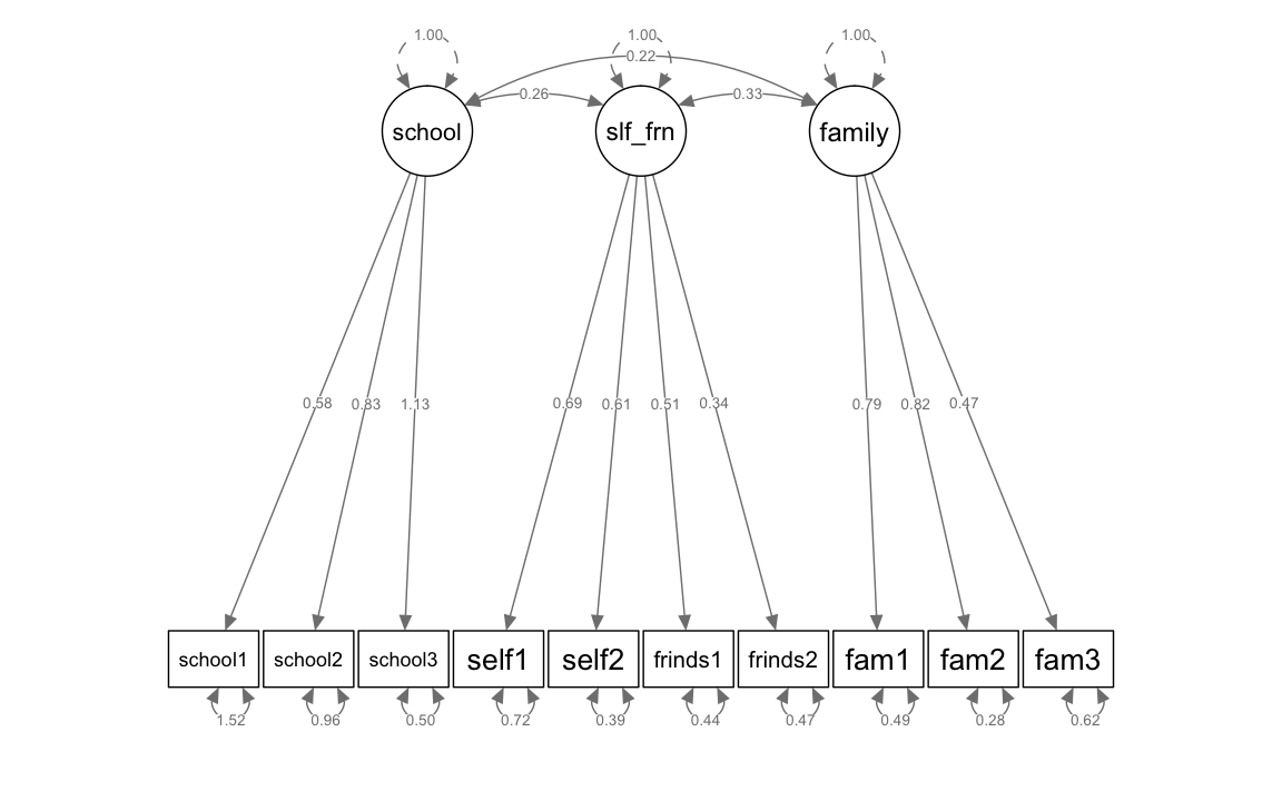
Model comparison of the 3-factor model and the alternative 3-factor model
A model comparison should now show that the 3-factor model and the restricted 4-factor model do have the same model fit, i.e. are identical:
anova(fit_mod3f, fit_mod4f_res)
#> Warning in lavTestLRT(object = new("lavaan", version = "0.6.4", call =
#> lavaan::lavaan(model = model_3f, : lavaan WARNING: some models have the
#> same degrees of freedom
#> Chi Square Difference Test
#>
#>               Df    AIC    BIC  Chisq Chisq diff Df diff Pr(>Chisq)
#> fit_mod3f     32 6929.6 7011.1 79.522
#> fit_mod4f_res 32 6929.6 7011.1 79.522 2.2919e-10       0
Exactly! (The very small number at Chisq diff is caused by minimal numerical inaccuracies in the ML estimation.)
Model comparison of the 3-factor model and the 4-factor model
Furthermore, we want to test the 3-factor model (it doesn’t matter which “version” we take, i.e. fit_mod3f or fit_mod4f_res) against the original 4-factor model.
This test examines whether the null hypothesis that the 3-factor model does not fit worse than the 4-factor model has to be rejected.
anova(fit_mod3f, fit_mod4f)
#> Chi Square Difference Test
#>
#>           Df    AIC    BIC  Chisq Chisq diff Df diff Pr(>Chisq)
#> fit_mod4f 29 6907.5 6999.6 51.433
#> fit_mod3f 32 6929.6 7011.1 79.522     28.089       3  3.479e-06 ***
#> ---
#> Signif. codes:  0 '***' 0.001 '**' 0.01 '*' 0.05 '.' 0.1 ' ' 1
The comparison is significant. The 3-factor model therefore fits the data significantly worse than the 4-factor model.
For the AIC, a value of 6907.52 was obtained for the 4-factor model and a value of 6929.609 for the 3-factor model. Thus, the 4-factor model should be preferred (smaller AIC).
A similar picture emerges for the BIC: BIC = 6999.593 for the 4-factor model and BIC = 7011.058 for the 3-factor model. Thus, even according to the more parsimonious BIC (favors models with fewer parameters as compared to the AIC), the 4-factor model should be selected.
10.1.6 Model with a second order factor
As we can see, the factors in the 4-factor model are all positively correlated and these correlations are also significant with one exception \((r_{SchoolSelf}=0.18, \; p = 0.052)\). This and the fact that life satisfaction in psychological research is conceptualized not only domain-specifically, but also (and even predominantly) globally, suggests that a 2nd order factor life satisfaction might exist. In other words: general life satisfaction factor might explain the inter-correlations among the domain-specific (first order) life satisfaction factors.
In CFA we can model such a second order factor. Another factor seems to make the model more complicated at first, but this can be misleading: In fact, in a model with one second order factor, there are two parameters less to be estimated than in a model with only four first order factors: Instead of six covariances among the factors, now four loadings (or three loadings and one second order factor variance) have to be estimated.
Model definition
model_4f_2order <-  "
school =~ school1 + school2 + school3
self =~ self1 + self2
friends =~ friends1 + friends2
family =~ fam1 + fam2 + fam3

# Second order factor life_satisfaction
life_satisfaction =~ school + self + friends + family
"
Model estimation
fit_mod4f_2order <- cfa(model_4f_2order, ls_clean)
summary(fit_mod4f_2order, fit.measures = TRUE, standardized = TRUE)
#> lavaan 0.6-4 ended normally after 67 iterations
#>
#>   Optimization method                           NLMINB
#>   Number of free parameters                         24
#>
#>   Number of observations                           255
#>
#>   Estimator                                         ML
#>   Model Fit Test Statistic                      53.372
#>   Degrees of freedom                                31
#>   P-value (Chi-square)                           0.008
#>
#> Model test baseline model:
#>
#>   Minimum Function Test Statistic              583.039
#>   Degrees of freedom                                45
#>   P-value                                        0.000
#>
#> User model versus baseline model:
#>
#>   Comparative Fit Index (CFI)                    0.958
#>   Tucker-Lewis Index (TLI)                       0.940
#>
#> Loglikelihood and Information Criteria:
#>
#>   Loglikelihood user model (H0)              -3428.730
#>   Loglikelihood unrestricted model (H1)      -3402.044
#>
#>   Number of free parameters                         24
#>   Akaike (AIC)                                6905.459
#>   Bayesian (BIC)                              6990.450
#>   Sample-size adjusted Bayesian (BIC)         6914.364
#>
#> Root Mean Square Error of Approximation:
#>
#>   RMSEA                                          0.053
#>   90 Percent Confidence Interval          0.027  0.077
#>   P-value RMSEA <= 0.05                          0.387
#>
#> Standardized Root Mean Square Residual:
#>
#>   SRMR                                           0.060
#>
#> Parameter Estimates:
#>
#>   Information                                 Expected
#>   Information saturated (h1) model          Structured
#>   Standard Errors                             Standard
#>
#> Latent Variables:
#>                        Estimate  Std.Err  z-value  P(>|z|)   Std.lv
#>   school =~
#>     school1               1.000                               0.555
#>     school2               1.439    0.261    5.508    0.000    0.799
#>     school3               2.118    0.449    4.713    0.000    1.175
#>   self =~
#>     self1                 1.000                               0.736
#>     self2                 0.924    0.153    6.040    0.000    0.680
#>   friends =~
#>     friends1              1.000                               0.662
#>     friends2              0.612    0.117    5.229    0.000    0.405
#>   family =~
#>     fam1                  1.000                               0.780
#>     fam2                  1.068    0.131    8.136    0.000    0.833
#>     fam3                  0.595    0.084    7.106    0.000    0.465
#>   life_satisfaction =~
#>     school                1.000                               0.322
#>     self                  2.720    0.985    2.763    0.006    0.661
#>     friends               3.397    1.250    2.717    0.007    0.917
#>     family                1.686    0.661    2.550    0.011    0.386
#>   Std.all
#>
#>     0.407
#>     0.622
#>     0.883
#>
#>     0.675
#>     0.777
#>
#>     0.792
#>     0.530
#>
#>     0.741
#>     0.849
#>     0.507
#>
#>     0.322
#>     0.661
#>     0.917
#>     0.386
#>
#> Variances:
#>                    Estimate  Std.Err  z-value  P(>|z|)   Std.lv  Std.all
#>    .school1           1.547    0.148   10.481    0.000    1.547    0.834
#>    .school2           1.011    0.139    7.278    0.000    1.011    0.613
#>    .school3           0.390    0.231    1.689    0.091    0.390    0.220
#>    .self1             0.647    0.100    6.442    0.000    0.647    0.544
#>    .self2             0.303    0.075    4.020    0.000    0.303    0.396
#>    .friends1          0.261    0.080    3.277    0.001    0.261    0.373
#>    .friends2          0.420    0.047    8.958    0.000    0.420    0.719
#>    .fam1              0.501    0.079    6.317    0.000    0.501    0.452
#>    .fam2              0.268    0.078    3.429    0.001    0.268    0.279
#>    .fam3              0.625    0.061   10.256    0.000    0.625    0.743
#>    .school            0.276    0.095    2.915    0.004    0.896    0.896
#>    .self              0.305    0.091    3.369    0.001    0.563    0.563
#>    .friends           0.070    0.106    0.661    0.509    0.159    0.159
#>    .family            0.518    0.097    5.360    0.000    0.851    0.851
#>     life_satisfctn    0.032    0.021    1.536    0.125    1.000    1.000
Visualizing the model
With standardized parameter estimates:
semPaths(fit_mod4f_2order, "std", weighted = FALSE, nCharNodes = 7,
         shapeMan = "rectangle", sizeMan = 8, sizeMan2 = 5)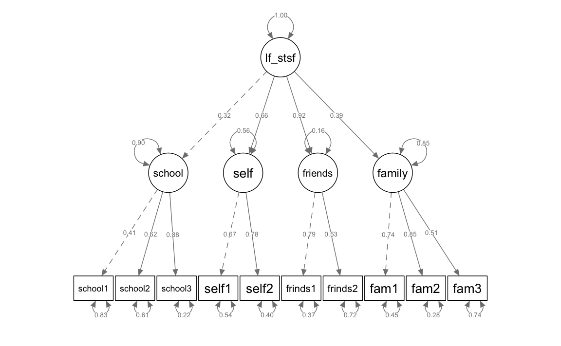
The parameter estimates show that the strongest standardized loading of the domain-specific (first order) factors is that of the friends factor, while the lowest is that of the school factor. Overall, the pattern of loadings is quite heterogeneous.
Model fit and model comparisons
CFI = 0.958 and NNFI/TLI = 0.94 are very similar to the 4-factor model. The RMSEA = 0.053 is slightly lower than with the 4-factor model and not significantly higher than 0.05 (90 %-CI [0.027; 0.077]).
Now we compare all three models (in ascending order with regard to the number of estimated parameters: 3-factor model, 4-factor model with second-order factor, 4-factor model) using sequential likelihood-ratio tests. The prerequisite for the validity of these tests is the nesting of restricted models (with fewer parameters) in models with fewer restrictions (with more parameters). For the 3-factor and the 4-factor models we have demonstrated the nesting above. But also the 4-factor model with a second-order factor is nested in the 4-factor model (because actually all models that have the same four first order factors are nested in this model since it is a saturated model at the level of latent variables).
anova(fit_mod3f, fit_mod4f_2order, fit_mod4f)
#> Chi Square Difference Test
#>
#>                  Df    AIC    BIC  Chisq Chisq diff Df diff Pr(>Chisq)
#> fit_mod4f        29 6907.5 6999.6 51.433
#> fit_mod4f_2order 31 6905.5 6990.4 53.372     1.9395       2     0.3792
#> fit_mod3f        32 6929.6 7011.1 79.522    26.1494       1   3.16e-07 ***
#> ---
#> Signif. codes:  0 '***' 0.001 '**' 0.01 '*' 0.05 '.' 0.1 ' ' 1
The model comparison shows that the 4-factor model with a second-order factor does not fit the data significantly worse than the less parsimonious 4-factor model (\(\Delta\chi^2=\) 1.9395, \(p =\) 0.3792). The second test, on the other hand, shows a significant model comparison of the 3-factor model with the 4-factor model with a second-order factor (\(\Delta\chi^2=\) 26.1494, \(p =\) 0).
The best of these three models is therefore the 4-factor model with a second order factor. This also has the lowest information criteria of all models (AIC = 6905.5, BIC = 6990.4).
10.2 Structural Equation Modelling (SEM)
10.2.1 Introduction
SEM represent a combination of CFA and regression models and allows to model complex regression structures (path models) at the level of latent variables. Indirect effects (mediation models) can also be estimated. The estimation theory does not differ from that of CFA.
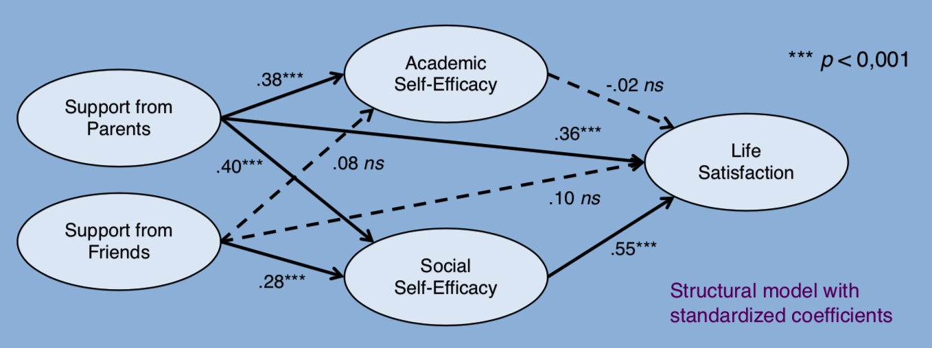
As an example we will study the effects of emotional support by parents and friends as experienced by adolescents on their life satisfaction. The two self-efficacy domains “academic self-efficacy” and “social self-efficacy” will serve as mediators for these effects. Both direct and indirect effects will be investigated.
Theoretical basis and hypotheses: Both parental support and support from friends have a positive effect on life satisfaction. In addition, it is known from self-efficacy research that experienced support has a positive effect on the experience of self-efficacy, and that this in turn is related to life satisfaction. An important question, however, concerns the differential effects resulting resulting when these constructs with their respective domains are considered simultaneously.
The assumed effects can be summarized in the following structural model:
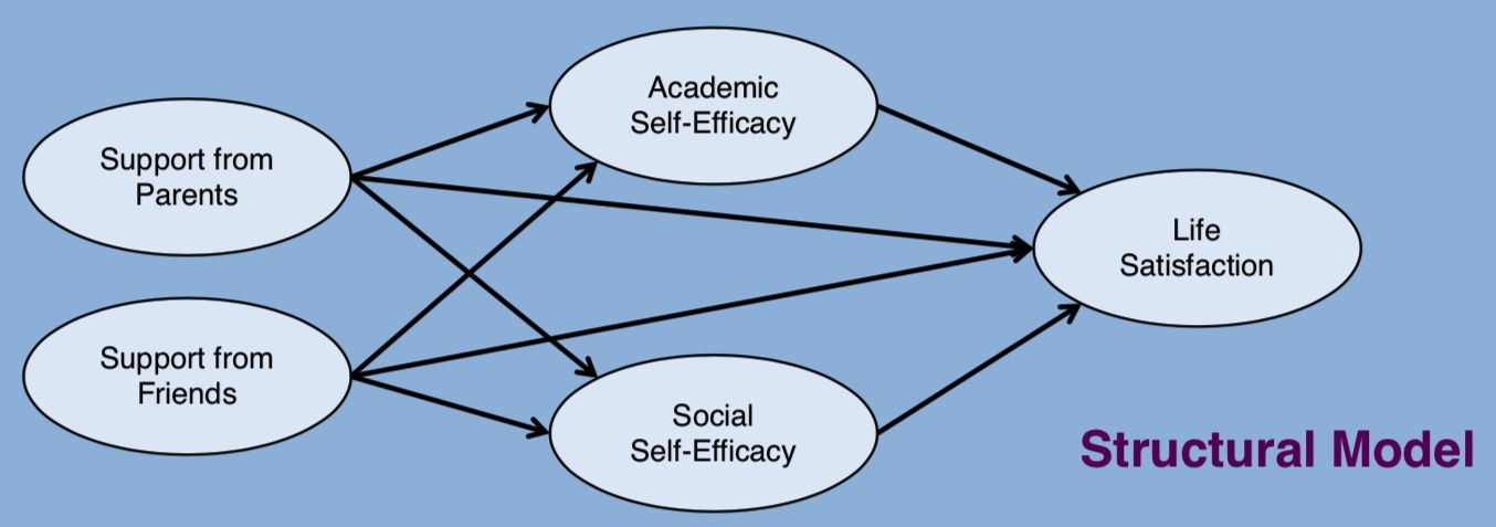
For the postulated structural model (relations between the latent variables) we need a measurement model (relations between the latent variables and the manifest variables, i.e. the factor structure). With a large number of measured variables the measurement model is often based “packages” of individual items rather than on the individual items themselves. Here we choose the “item-to-construct balance approach” to packaging (Little et al., 2002), in which individual items representing a certain construct are combined in such a way that the “packed” manifest variables load as homogeneously as possible on the respective latent factor. It is generally recommended to use three to four parcels per latent variable.
The following parcels were built:
Emotional support from parents (6 items): 3 parcels of 2 items (sup_parents_p1, sup_parents_p2, sup_parents_p3)
Emotional support from friends (6 items): 3 parcels of 2 items (sup_friends_p1, sup_friends_p2, sup_friends_p3)
Academic self-efficacy (20 items): 2 parcels of 7 items & 1 parcel of 6 items (se_acad_p1, se_acad_p2, se_acad_p3)
Social self-efficacy (16 items): 2 parcels of 5 items & 1 parcel of 6 items (se_social_p1, se_social_p2, se_social_p3)
Life satisfaction (11 items): 2 parcels of 4 items & 1 parcel of 3 items (ls_p1, ls_p2, ls_p3)
The SEM analysis is carried out in three steps:
We start with the measurement model. The measurement model is a multi-construct CFA with intercorrelations of all latent variables.
Then we consider the entire structural equation model (measurement and structural model combined).
In the last step we will show how to explicitly define indirect and total effects within the SEM.
10.2.2 Importing the data
data_sem <- read_csv("data/sem_data.csv") %>%
  mutate(region = as.factor(region),
         sex = as.factor(sex))
#> Parsed with column specification:
#> cols(
#>   ID = col_double(),
#>   region = col_character(),
#>   sex = col_character(),
#>   age = col_double(),
#>   se_acad_p1 = col_double(),
#>   se_acad_p2 = col_double(),
#>   se_acad_p3 = col_double(),
#>   se_social_p1 = col_double(),
#>   se_social_p2 = col_double(),
#>   se_social_p3 = col_double(),
#>   sup_friends_p1 = col_double(),
#>   sup_friends_p2 = col_double(),
#>   sup_friends_p3 = col_double(),
#>   sup_parents_p1 = col_double(),
#>   sup_parents_p2 = col_double(),
#>   sup_parents_p3 = col_double(),
#>   ls_p1 = col_double(),
#>   ls_p2 = col_double(),
#>   ls_p3 = col_double()
#> )
As above with the CFA, we remove all persons with observations outside +/- 3 SD of the mean on one or more variables:
keep <- function(x) {
  (x >= mean(x, na.rm = TRUE) - 3 * sd(x, na.rm = TRUE)) &
    (x <= mean(x, na.rm = TRUE) + 3 * sd(x, na.rm = TRUE))
}

data_clean <- data_sem %>%
  filter(
      keep(se_acad_p1) &
      keep(se_acad_p2) &
      keep(se_acad_p3) &
      keep(se_social_p1) &
      keep(se_social_p2) &
      keep(se_social_p3) &
      keep(sup_parents_p1) &
      keep(sup_parents_p2) &
      keep(sup_parents_p3) &
      keep(sup_friends_p1) &
      keep(sup_friends_p2) &
      keep(sup_friends_p3) &
      keep(ls_p1) &
      keep(ls_p2) &
      keep(ls_p3))

data_clean
#> # A tibble: 255 x 19
#>      ID region sex     age se_acad_p1 se_acad_p2 se_acad_p3 se_social_p1
#>   <dbl> <fct>  <fct> <dbl>      <dbl>      <dbl>      <dbl>        <dbl>
#> 1     1 west   fema…    13       4.86       5.57       4.5          5.8
#> 2     2 west   male     14       4.57       4.29       4.67         5
#> 3    10 west   fema…    14       4.14       6.14       5.33         5.2
#> 4    11 west   fema…    14       5          5.43       4.83         6.4
#> 5    12 west   fema…    14       5.17       5.6        4.8          5.25
#> 6    14 west   male     14       4.86       4.86       4.17         5.2
#> # … with 249 more rows, and 11 more variables: se_social_p2 <dbl>,
#> #   se_social_p3 <dbl>, sup_friends_p1 <dbl>, sup_friends_p2 <dbl>,
#> #   sup_friends_p3 <dbl>, sup_parents_p1 <dbl>, sup_parents_p2 <dbl>,
#> #   sup_parents_p3 <dbl>, ls_p1 <dbl>, ls_p2 <dbl>, ls_p3 <dbl>
10.2.3 Measurement model
In the measurement model, the relationships between the latent variables (factors) and the manifest variables are defined. We are already familiar with the lavaan model definition from the CFA example above.
Error variances of the observed variables and variances of the exogenous latent variables do not have to be explicitly specified.
Operator for the measuring model:
=~(“is measured by…”)
model_measurement <- "
# Measurement model
SUP_Parents =~ sup_parents_p1 + sup_parents_p2 + sup_parents_p3
SUP_Friends =~ sup_friends_p1 + sup_friends_p2 + sup_friends_p3
SE_Academic =~ se_acad_p1 + se_acad_p2 + se_acad_p3
SE_Social =~ se_social_p1 + se_social_p2 + se_social_p3
LS  =~ ls_p1 + ls_p2 + ls_p3
"
Model estimation
The function sem() is applied to the model model_measurement specified above, the results are stored in an object (here with the name fit_measurement). We could also use cfa() here. The two functions differ only slightly in their default settings and are both equally suitable for estimating measurement models.
fit_measurement <- sem(model_measurement, data = data_clean)
summary(fit_measurement, fit.measures = TRUE, standardized = TRUE)
#> lavaan 0.6-4 ended normally after 49 iterations
#>
#>   Optimization method                           NLMINB
#>   Number of free parameters                         40
#>
#>   Number of observations                           255
#>
#>   Estimator                                         ML
#>   Model Fit Test Statistic                     212.282
#>   Degrees of freedom                                80
#>   P-value (Chi-square)                           0.000
#>
#> Model test baseline model:
#>
#>   Minimum Function Test Statistic             2238.104
#>   Degrees of freedom                               105
#>   P-value                                        0.000
#>
#> User model versus baseline model:
#>
#>   Comparative Fit Index (CFI)                    0.938
#>   Tucker-Lewis Index (TLI)                       0.919
#>
#> Loglikelihood and Information Criteria:
#>
#>   Loglikelihood user model (H0)              -3510.025
#>   Loglikelihood unrestricted model (H1)      -3403.884
#>
#>   Number of free parameters                         40
#>   Akaike (AIC)                                7100.051
#>   Bayesian (BIC)                              7241.701
#>   Sample-size adjusted Bayesian (BIC)         7114.892
#>
#> Root Mean Square Error of Approximation:
#>
#>   RMSEA                                          0.081
#>   90 Percent Confidence Interval          0.067  0.094
#>   P-value RMSEA <= 0.05                          0.000
#>
#> Standardized Root Mean Square Residual:
#>
#>   SRMR                                           0.062
#>
#> Parameter Estimates:
#>
#>   Information                                 Expected
#>   Information saturated (h1) model          Structured
#>   Standard Errors                             Standard
#>
#> Latent Variables:
#>                    Estimate  Std.Err  z-value  P(>|z|)   Std.lv  Std.all
#>   SUP_Parents =~
#>     sup_parents_p1    1.000                               0.767    0.834
#>     sup_parents_p2    1.127    0.070   16.029    0.000    0.865    0.898
#>     sup_parents_p3    1.029    0.072   14.254    0.000    0.789    0.792
#>   SUP_Friends =~
#>     sup_friends_p1    1.000                               0.816    0.867
#>     sup_friends_p2    0.836    0.053   15.777    0.000    0.682    0.846
#>     sup_friends_p3    0.924    0.059   15.584    0.000    0.753    0.835
#>   SE_Academic =~
#>     se_acad_p1        1.000                               0.651    0.856
#>     se_acad_p2        0.844    0.055   15.323    0.000    0.550    0.837
#>     se_acad_p3        1.000    0.066   15.063    0.000    0.651    0.824
#>   SE_Social =~
#>     se_social_p1      1.000                               0.558    0.816
#>     se_social_p2      0.976    0.065   15.072    0.000    0.544    0.879
#>     se_social_p3      0.968    0.078   12.398    0.000    0.540    0.732
#>   LS =~
#>     ls_p1             1.000                               0.527    0.639
#>     ls_p2             0.877    0.097    9.031    0.000    0.462    0.772
#>     ls_p3             0.907    0.117    7.775    0.000    0.478    0.609
#>
#> Covariances:
#>                    Estimate  Std.Err  z-value  P(>|z|)   Std.lv  Std.all
#>   SUP_Parents ~~
#>     SUP_Friends       0.104    0.045    2.322    0.020    0.167    0.167
#>     SE_Academic       0.199    0.039    5.090    0.000    0.397    0.397
#>     SE_Social         0.191    0.035    5.503    0.000    0.446    0.446
#>     LS                0.248    0.041    6.014    0.000    0.613    0.613
#>   SUP_Friends ~~
#>     SE_Academic       0.078    0.038    2.044    0.041    0.147    0.147
#>     SE_Social         0.159    0.035    4.542    0.000    0.350    0.350
#>     LS                0.148    0.037    4.021    0.000    0.345    0.345
#>   SE_Academic ~~
#>     SE_Social         0.226    0.032    7.013    0.000    0.621    0.621
#>     LS                0.165    0.032    5.158    0.000    0.480    0.480
#>   SE_Social ~~
#>     LS                0.215    0.033    6.546    0.000    0.731    0.731
#>
#> Variances:
#>                    Estimate  Std.Err  z-value  P(>|z|)   Std.lv  Std.all
#>    .sup_parents_p1    0.258    0.033    7.799    0.000    0.258    0.305
#>    .sup_parents_p2    0.180    0.034    5.342    0.000    0.180    0.194
#>    .sup_parents_p3    0.369    0.042    8.826    0.000    0.369    0.372
#>    .sup_friends_p1    0.219    0.033    6.577    0.000    0.219    0.248
#>    .sup_friends_p2    0.185    0.025    7.380    0.000    0.185    0.285
#>    .sup_friends_p3    0.246    0.032    7.724    0.000    0.246    0.303
#>    .se_acad_p1        0.155    0.022    7.005    0.000    0.155    0.268
#>    .se_acad_p2        0.129    0.017    7.607    0.000    0.129    0.299
#>    .se_acad_p3        0.200    0.025    7.983    0.000    0.200    0.321
#>    .se_social_p1      0.156    0.019    8.098    0.000    0.156    0.334
#>    .se_social_p2      0.087    0.014    6.037    0.000    0.087    0.227
#>    .se_social_p3      0.253    0.027    9.529    0.000    0.253    0.465
#>    .ls_p1             0.402    0.043    9.358    0.000    0.402    0.592
#>    .ls_p2             0.145    0.021    6.991    0.000    0.145    0.404
#>    .ls_p3             0.387    0.040    9.651    0.000    0.387    0.629
#>     SUP_Parents       0.588    0.075    7.811    0.000    1.000    1.000
#>     SUP_Friends       0.665    0.081    8.258    0.000    1.000    1.000
#>     SE_Academic       0.424    0.052    8.096    0.000    1.000    1.000
#>     SE_Social         0.311    0.041    7.539    0.000    1.000    1.000
#>     LS                0.278    0.054    5.124    0.000    1.000    1.000
Path diagram
cols <- wes_palette(name = "Moonrise2", n = 4, type = "discrete")
colorlist <- list(man = cols[2], lat = cols[3])

semPaths(fit_measurement, what = "col", whatLabels = "std", style = "mx",
         color = colorlist, rotation =1 , layout = "spring",  nCharNodes = 7,
         shapeMan = "rectangle", sizeMan = 8, sizeMan2 = 5)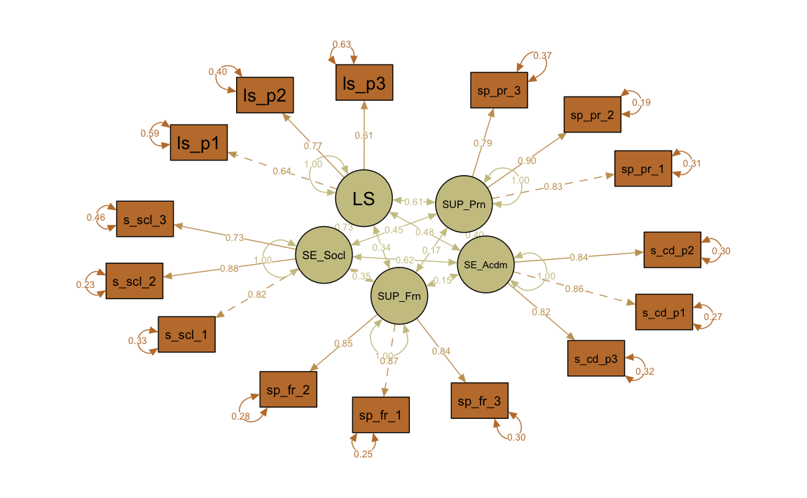
As can be seen from the output and the path diagram the standardized loadings are all relatively high and also homogeneous. The factor correlations of this multi-construct measurement model are between \(r = 0.147\) (SUP_Friends \(\leftrightarrow\) SE_Academic) and \(r = 0.731\) (SE_Social \(\leftrightarrow\) LS).
Global model fit is not really good (CFI = 0.938, NNFI/TLI = 0.919, RMSEA = 0.081, 90 %-CI: [0.067; 0.094]) but can still be seen as acceptable according to commonly accepted criteria.
In order to determine where problems exist in the model fit, we can first consider the standardized residual variance-covariance matrix:
resid(fit_measurement, type = "standardized")$cov
#>                sp_p_1 sp_p_2 sp_p_3 sp_f_1 sp_f_2 sp_f_3 s_cd_1 s_cd_2
#> sup_parents_p1  0.000
#> sup_parents_p2  2.058  0.000
#> sup_parents_p3 -1.325 -0.681  0.000
#> sup_friends_p1 -0.206 -0.825 -3.968  0.000
#> sup_friends_p2  1.598  1.876 -0.832  0.155  0.000
#> sup_friends_p3  1.786  0.669 -0.982  1.531 -1.703  0.000
#> se_acad_p1      0.191 -1.333  1.144 -0.342  0.697  0.926  0.000
#> se_acad_p2      0.663  0.536  1.354  1.240  1.536  1.042 -1.790  0.000
#> se_acad_p3     -0.765 -1.328  0.896 -2.929 -1.029 -1.327  1.150  0.467
#> se_social_p1    0.707  0.492  1.563 -3.450 -1.276 -1.381  3.946  2.006
#> se_social_p2   -0.009  0.130 -0.141  0.476  1.673  1.179 -1.211 -0.998
#> se_social_p3   -1.222 -0.996 -1.217  2.087  0.317  0.267 -0.661  1.423
#> ls_p1          -1.903 -1.605  0.875 -4.028 -1.760 -2.144 -0.497  3.392
#> ls_p2          -1.534 -2.798 -0.873  0.797  4.307  2.353 -3.750 -1.253
#> ls_p3           2.532  3.775  4.927 -1.629  0.172 -0.948  2.607  3.695
#>                s_cd_3 s_sc_1 s_sc_2 s_sc_3 ls_p1  ls_p2  ls_p3
#> sup_parents_p1
#> sup_parents_p2
#> sup_parents_p3
#> sup_friends_p1
#> sup_friends_p2
#> sup_friends_p3
#> se_acad_p1
#> se_acad_p2
#> se_acad_p3      0.000
#> se_social_p1    0.754  0.000
#> se_social_p2   -3.101  0.651  0.000
#> se_social_p3   -0.724 -2.033  1.227  0.000
#> ls_p1           1.549 -1.480 -2.091 -0.892  0.000
#> ls_p2          -3.683  1.030  2.698  2.450  2.101  0.000
#> ls_p3           2.661 -1.025 -1.797 -1.568  1.913 -4.710  0.000
This shows that the variance-covariance matrix implied by the model deviates significantly from the empirical variance-covariance matrix at many points in the model. An accumulation of very high standardized residual covariances can be seen e.g. with respect to the ls_p3 parcel.
Modification indices
Another possibility for local fit diagnostics is offered by modification indices. These indicate which additional model parameters would result in a significant fit improvement (in terms of a reduction of \(\chi^2\) by the value of the corresponding MI). We will only display the MI \(\geq 5\), since usually only those are considered substantial.
modindices(fit_measurement, standardized = FALSE, minimum.value = 5)
#>                lhs op            rhs     mi    epc
#> 46     SUP_Parents =~ sup_friends_p1  5.806 -0.127
#> 56     SUP_Parents =~          ls_p2 10.805 -0.241
#> 57     SUP_Parents =~          ls_p3 26.005  0.450
#> 60     SUP_Friends =~ sup_parents_p3  7.412 -0.154
#> 63     SUP_Friends =~     se_acad_p3  6.796 -0.115
#> 64     SUP_Friends =~   se_social_p1  9.715 -0.132
#> 67     SUP_Friends =~          ls_p1 11.286 -0.221
#> 68     SUP_Friends =~          ls_p2 15.297  0.197
#> 76     SE_Academic =~   se_social_p1 13.160  0.258
#> 77     SE_Academic =~   se_social_p2 11.197 -0.219
#> 80     SE_Academic =~          ls_p2 21.078 -0.334
#> 81     SE_Academic =~          ls_p3 14.463  0.339
#> 92       SE_Social =~          ls_p2 10.964  0.473
#> 97              LS =~ sup_friends_p1  7.059 -0.233
#> 98              LS =~ sup_friends_p2  5.678  0.182
#> 101             LS =~     se_acad_p2  7.019  0.193
#> 133 sup_parents_p3 ~~ sup_friends_p1  9.759 -0.075
#> 144 sup_parents_p3 ~~          ls_p3  8.031  0.079
#> 150 sup_friends_p1 ~~   se_social_p1  7.693 -0.045
#> 152 sup_friends_p1 ~~   se_social_p3 16.979  0.080
#> 164 sup_friends_p2 ~~          ls_p2  5.829  0.035
#> 177     se_acad_p1 ~~   se_social_p1 12.599  0.048
#> 180     se_acad_p1 ~~          ls_p1  6.038 -0.050
#> 187     se_acad_p2 ~~          ls_p1  7.547  0.049
#> 206   se_social_p3 ~~          ls_p2  5.442  0.036
#> 208          ls_p1 ~~          ls_p2  5.076  0.063
#> 210          ls_p2 ~~          ls_p3 17.111 -0.105
A total of 27 modification indices are displayed. They refer either to possible cross-loadings (e.g. SUP_Parents =~ ls_p3: MI = 26.005) or to residual covariances between manifest variables (e.g. sup_friends_p1 ~~ se_social_p3: MI = 16.979). For theoretical reasons the addition of cross-loadings and of residual covariances (especially across different latent variables) is not recommended.
Such model fit problems often arise in self-report studies. Individual differences in scale use (response styles) can play a role: These can lead to generally increased correlations among the variables, which may not be adequately taken into account in a multi-construct measurement model. There are approaches (definition of method and response style factors) to deal with this issue.
Another reason for the model-fit problems in this study could be the general similarity of the constructs investigated with respect to life domains. For example, there are life satisfaction items with respect to friends, but the friends context also plays an important role for the items for social self-efficacy and, of course, for support received from friends.
Since the model fit is still acceptable, we continue to work with this measurement model. In the next step we will model the effects among latent variables in order to test our theoretical assumptions (structural model).
10.2.4 Structural model
Model definition
The structural model represents the relationships/effects among the latent variables. It is added to the measurement model definitions:
model <- "
# Measurement model
SUP_Parents =~ sup_parents_p1 + sup_parents_p2 + sup_parents_p3
SUP_Friends =~ sup_friends_p1 + sup_friends_p2 + sup_friends_p3
SE_Academic =~ se_acad_p1 + se_acad_p2 + se_acad_p3
SE_Social =~ se_social_p1 + se_social_p2 + se_social_p3
LS  =~ ls_p1 + ls_p2 + ls_p3

# Structural model
# Regressions
SE_Academic ~ SUP_Parents + SUP_Friends
SE_Social ~ SUP_Parents + SUP_Friends
LS ~ SE_Academic + SE_Social + SUP_Parents + SUP_Friends

# Residual covariances
SE_Academic ~~ SE_Social
"
Operator for the structural model (regressions of latent variables):
~(“is predicted by…”)Operator for (residual) variances and covariances:
~~(for variances, the same variable appears on the left and right; for covariances, different variables). As in the measurement model (CFA), variances and covariances of exogenous latent variables do not have to be specified (are automatically estimated). The residual variances of endogenous latent variables are also estimated automatically.
Therefore we only have to specify one parameter using ~~: In this model we have two parallel latent mediator variables (SE_Academic and SE_Social) which have no effects on each other. However, it can be assumed that these two variables (or rather their residuals) co-vary since a general self-efficacy component is likely (cf. also the correlation of \(r=0.621\) in the measurement model above). Since SE_Academic and SE_Social are endogenous latent variables (both are predicted by both SUP_Parents and SUP_Friends), a residual covariance \(\psi =\) SE_Academic ~~ SE_Social must be specified.
Model estimation
fit <- sem(model, data = data_clean)
summary(fit, fit.measures = TRUE, standardized = TRUE)
#> lavaan 0.6-4 ended normally after 46 iterations
#>
#>   Optimization method                           NLMINB
#>   Number of free parameters                         40
#>
#>   Number of observations                           255
#>
#>   Estimator                                         ML
#>   Model Fit Test Statistic                     212.282
#>   Degrees of freedom                                80
#>   P-value (Chi-square)                           0.000
#>
#> Model test baseline model:
#>
#>   Minimum Function Test Statistic             2238.104
#>   Degrees of freedom                               105
#>   P-value                                        0.000
#>
#> User model versus baseline model:
#>
#>   Comparative Fit Index (CFI)                    0.938
#>   Tucker-Lewis Index (TLI)                       0.919
#>
#> Loglikelihood and Information Criteria:
#>
#>   Loglikelihood user model (H0)              -3510.025
#>   Loglikelihood unrestricted model (H1)      -3403.884
#>
#>   Number of free parameters                         40
#>   Akaike (AIC)                                7100.051
#>   Bayesian (BIC)                              7241.701
#>   Sample-size adjusted Bayesian (BIC)         7114.892
#>
#> Root Mean Square Error of Approximation:
#>
#>   RMSEA                                          0.081
#>   90 Percent Confidence Interval          0.067  0.094
#>   P-value RMSEA <= 0.05                          0.000
#>
#> Standardized Root Mean Square Residual:
#>
#>   SRMR                                           0.062
#>
#> Parameter Estimates:
#>
#>   Information                                 Expected
#>   Information saturated (h1) model          Structured
#>   Standard Errors                             Standard
#>
#> Latent Variables:
#>                    Estimate  Std.Err  z-value  P(>|z|)   Std.lv  Std.all
#>   SUP_Parents =~
#>     sup_parents_p1    1.000                               0.767    0.834
#>     sup_parents_p2    1.127    0.070   16.029    0.000    0.865    0.898
#>     sup_parents_p3    1.029    0.072   14.254    0.000    0.789    0.792
#>   SUP_Friends =~
#>     sup_friends_p1    1.000                               0.816    0.867
#>     sup_friends_p2    0.836    0.053   15.777    0.000    0.682    0.846
#>     sup_friends_p3    0.924    0.059   15.584    0.000    0.753    0.835
#>   SE_Academic =~
#>     se_acad_p1        1.000                               0.651    0.856
#>     se_acad_p2        0.844    0.055   15.323    0.000    0.550    0.837
#>     se_acad_p3        1.000    0.066   15.063    0.000    0.651    0.824
#>   SE_Social =~
#>     se_social_p1      1.000                               0.558    0.816
#>     se_social_p2      0.976    0.065   15.072    0.000    0.544    0.879
#>     se_social_p3      0.968    0.078   12.398    0.000    0.540    0.732
#>   LS =~
#>     ls_p1             1.000                               0.527    0.639
#>     ls_p2             0.877    0.097    9.031    0.000    0.462    0.772
#>     ls_p3             0.907    0.117    7.775    0.000    0.478    0.609
#>
#> Regressions:
#>                    Estimate  Std.Err  z-value  P(>|z|)   Std.lv  Std.all
#>   SE_Academic ~
#>     SUP_Parents       0.326    0.060    5.450    0.000    0.384    0.384
#>     SUP_Friends       0.066    0.054    1.229    0.219    0.083    0.083
#>   SE_Social ~
#>     SUP_Parents       0.290    0.050    5.822    0.000    0.399    0.399
#>     SUP_Friends       0.194    0.045    4.278    0.000    0.284    0.284
#>   LS ~
#>     SE_Academic      -0.014    0.068   -0.211    0.833   -0.018   -0.018
#>     SE_Social         0.519    0.099    5.260    0.000    0.549    0.549
#>     SUP_Parents       0.247    0.052    4.772    0.000    0.359    0.359
#>     SUP_Friends       0.061    0.042    1.461    0.144    0.095    0.095
#>
#> Covariances:
#>                    Estimate  Std.Err  z-value  P(>|z|)   Std.lv  Std.all
#>  .SE_Academic ~~
#>    .SE_Social         0.153    0.025    6.051    0.000    0.542    0.542
#>   SUP_Parents ~~
#>     SUP_Friends       0.104    0.045    2.322    0.020    0.167    0.167
#>
#> Variances:
#>                    Estimate  Std.Err  z-value  P(>|z|)   Std.lv  Std.all
#>    .sup_parents_p1    0.258    0.033    7.799    0.000    0.258    0.305
#>    .sup_parents_p2    0.180    0.034    5.342    0.000    0.180    0.194
#>    .sup_parents_p3    0.369    0.042    8.826    0.000    0.369    0.372
#>    .sup_friends_p1    0.219    0.033    6.577    0.000    0.219    0.248
#>    .sup_friends_p2    0.185    0.025    7.380    0.000    0.185    0.285
#>    .sup_friends_p3    0.246    0.032    7.724    0.000    0.246    0.303
#>    .se_acad_p1        0.155    0.022    7.005    0.000    0.155    0.268
#>    .se_acad_p2        0.129    0.017    7.607    0.000    0.129    0.299
#>    .se_acad_p3        0.200    0.025    7.983    0.000    0.200    0.321
#>    .se_social_p1      0.156    0.019    8.098    0.000    0.156    0.334
#>    .se_social_p2      0.087    0.014    6.037    0.000    0.087    0.227
#>    .se_social_p3      0.253    0.027    9.529    0.000    0.253    0.465
#>    .ls_p1             0.402    0.043    9.358    0.000    0.402    0.592
#>    .ls_p2             0.145    0.021    6.991    0.000    0.145    0.404
#>    .ls_p3             0.387    0.040    9.651    0.000    0.387    0.629
#>     SUP_Parents       0.588    0.075    7.811    0.000    1.000    1.000
#>     SUP_Friends       0.665    0.081    8.258    0.000    1.000    1.000
#>    .SE_Academic       0.354    0.045    7.849    0.000    0.835    0.835
#>    .SE_Social         0.225    0.031    7.165    0.000    0.723    0.723
#>    .LS                0.098    0.025    3.923    0.000    0.354    0.354
The model fit is exactly the same! We have already seen above that we have just as many parameters and degrees of freedom in the overall model as in the measurement model.
This means that the structural model is saturated!
In the measurement model we had 15 variance and covariance parameters of the latent variables, so the variance-covariance matrix of the latent variables (with 5 x 6/2 = 15 elements) was complete and unrestricted. We now also have 15 parameters in the structural model. The parameters of the structural model are estimable and we can thus check our postulated effects, but this part of the overall model is just identified (since \(n_{Info} = n_{Par}\) with regard to the latent variables) and thus does not contribute to the model fit of the overall model! In other words: We cannot check whether the structural model fits our data well, only the fit of the measurement model can be tested.
Interpretation of the estimated structural coefficients: Of the 8 postulated structural paths, 5 are significant and go in the expected direction. Not significant are the effects of SUP_Friends on SE_Academic (Std.all \(= 0.083,\ p = 0.219\)), from SE_Academic to LS (Std.all \(= -0.018,\ p = 0.833\)), and from SUP_Friends to LS (Stds.all \(= 0.095,\ p = 0.144\)).
It is particularly striking that the perceived support by the parents has a substantial direct effect on satisfaction, whereas the direct effect of the perceived support by the friends is not significant. It is also interesting that the academic self-efficacy no longer has a significant effect on satisfaction when social self-efficacy is held constant, even though the correlation between the two latent variables SE_Academic and LS was substantial in the measurement model (see above \(r = 0.480,\ p < 0.001\)).
Path diagram
Path diagram with non-standardized parameter estimates (layout = 'tree2'):
semPaths(fit, what = "col", whatLabels = "par", style = "mx", color = colorlist,
         rotation = 2, layout = "tree2", mar = c(1, 2, 1, 2), nCharNodes = 7,
         shapeMan = "rectangle", sizeMan = 8, sizeMan2 = 5)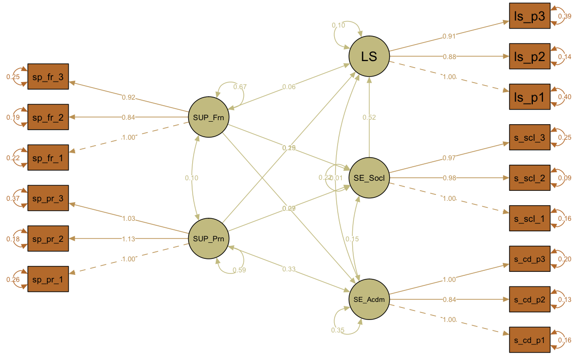
Path diagram with non-standardized parameter estimates (layout = 'spring'):
semPaths(fit, what = "col", whatLabels = "std", style = "mx",  color = colorlist,
         rotation =1 , layout = "spring",  nCharNodes = 7, shapeMan = "rectangle",
         sizeMan = 8, sizeMan2 = 5)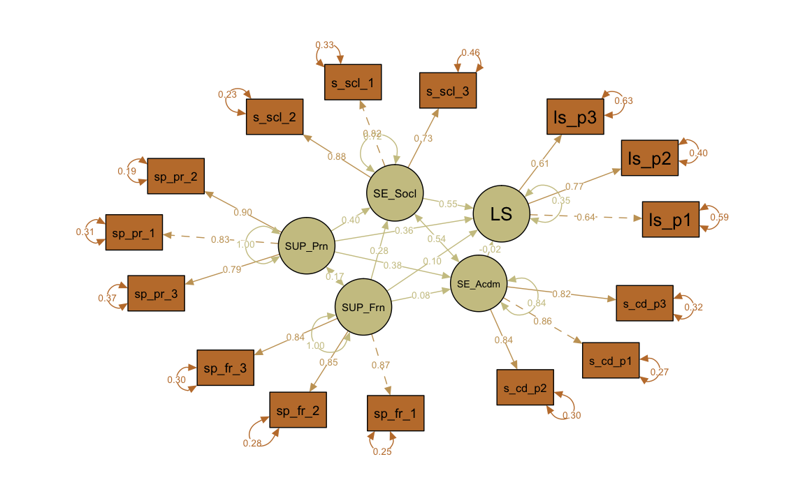
Calculation of standardized indirect and total effects
Use the Std.all estimates!
Specific indirect effects
SUP_Parents\(\rightarrow\)SE_Academic\(\rightarrow\)LS:
\(0.384 \cdot -0.018 = -0.007\)
\(~\)
SUP_Parents\(\rightarrow\)SE_Social\(\rightarrow\)LS:
\(0.399 \cdot 0.549 = 0.219\)
\(~\)
SUP_Friends\(\rightarrow\)SE_Academic\(\rightarrow\)LS:
\(0.083 \cdot -0.018 = -0.001\)
\(~\)
SUP_Friends\(\rightarrow\)SE_Social\(\rightarrow\)LS:
\(0.284 \cdot 0.549 = 0.156\)
\(~\)
Total indirect effects
SUP_Parents\(\rightarrow\)LSthroughSE_AcademicandSE_Social:**
\(0.384 \cdot -0.018 + 0.399 \cdot 0.549 = 0.212\)
\(~\)
SUP_Friends\(\rightarrow\)LSthroughSE_AcademicandSE_Social:
\(0.083 \cdot -0.018 + 0.284 \cdot 0.549 = 0.154\)
\(~\)
Total effects
SUP_Parents\(\rightarrow\)LS:
\(0.384 \cdot -0.018 + 0.399 \cdot 0.549 + 0.359 = 0.571\)
\(~\)
SUP_Friends\(\rightarrow\)LS:
\(0.083 \cdot -0.018 + 0.284 \cdot 0.549 + 0.095 = 0.249\)
\(~\)
We can also estimate indirect and total effects in lavaan and get significance tests for them. This is our last step in the analysis of this SEM.
Significance tests for indirect and total effects
With one or more latent mediator variables present in the structural model the SEM turns into a latent mediation analysis. To estimate indirect and total effects, the parameters of the structural model must first be explicitly named in the model definition (multiplication of predictors with b1, b2, b3, etc.).
Specific and total indirect effects can then be defined as products (or sum of products) of the path parameters (operator:
:=)Total effects can be defined equally as the sum of indirect and direct effects
When indirect and total effects are defined the model should always be estimated using the se = bootstrap option. The reason for this is that other than the path coefficients themselves indirect effects (products of path coefficients) are not asymptotically normally distributed and therefore the z- or Wald-approximation should not be used for these defined parameters.
model_mediation <- '
# Measurement model
SUP_Parents =~ sup_parents_p1 + sup_parents_p2 + sup_parents_p3
SUP_Friends =~ sup_friends_p1 + sup_friends_p2 + sup_friends_p3
SE_Academic =~ se_acad_p1 + se_acad_p2 + se_acad_p3
SE_Social =~ se_social_p1 + se_social_p2 + se_social_p3
LS  =~ ls_p1 + ls_p2 + ls_p3

# Structural model
# Regressions
SE_Academic ~ b1*SUP_Parents + b3*SUP_Friends
SE_Social ~ b2*SUP_Parents + b4*SUP_Friends
LS ~ b5*SUP_Parents + b6*SUP_Friends + b7*SE_Academic + b8*SE_Social

# Residual covariances
SE_Academic ~~ SE_Social

# Indirect effects
b1b7 := b1*b7
b2b8 := b2*b8
totalind_eltern := b1*b7 + b2*b8
b3b7 := b3*b7
b4b8 := b4*b8
totalind_freunde := b3*b7 + b4*b8

# Total effects
total_eltern := b1*b7 + b2*b8 + b5
total_freunde := b3*b7 + b4*b8 + b6
'

fit_mediation <- sem(model_mediation, data = data_clean, se = "bootstrap")
summary(fit_mediation, fit.measures = TRUE, standardized = TRUE)
#> lavaan 0.6-4 ended normally after 46 iterations
#>
#>   Optimization method                           NLMINB
#>   Number of free parameters                         40
#>
#>   Number of observations                           255
#>
#>   Estimator                                         ML
#>   Model Fit Test Statistic                     212.282
#>   Degrees of freedom                                80
#>   P-value (Chi-square)                           0.000
#>
#> Model test baseline model:
#>
#>   Minimum Function Test Statistic             2238.104
#>   Degrees of freedom                               105
#>   P-value                                        0.000
#>
#> User model versus baseline model:
#>
#>   Comparative Fit Index (CFI)                    0.938
#>   Tucker-Lewis Index (TLI)                       0.919
#>
#> Loglikelihood and Information Criteria:
#>
#>   Loglikelihood user model (H0)              -3510.025
#>   Loglikelihood unrestricted model (H1)      -3403.884
#>
#>   Number of free parameters                         40
#>   Akaike (AIC)                                7100.051
#>   Bayesian (BIC)                              7241.701
#>   Sample-size adjusted Bayesian (BIC)         7114.892
#>
#> Root Mean Square Error of Approximation:
#>
#>   RMSEA                                          0.081
#>   90 Percent Confidence Interval          0.067  0.094
#>   P-value RMSEA <= 0.05                          0.000
#>
#> Standardized Root Mean Square Residual:
#>
#>   SRMR                                           0.062
#>
#> Parameter Estimates:
#>
#>   Standard Errors                            Bootstrap
#>   Number of requested bootstrap draws             1000
#>   Number of successful bootstrap draws            1000
#>
#> Latent Variables:
#>                    Estimate  Std.Err  z-value  P(>|z|)   Std.lv  Std.all
#>   SUP_Parents =~
#>     sup_parents_p1    1.000                               0.767    0.834
#>     sup_parents_p2    1.127    0.075   15.098    0.000    0.865    0.898
#>     sup_parents_p3    1.029    0.094   10.983    0.000    0.789    0.792
#>   SUP_Friends =~
#>     sup_friends_p1    1.000                               0.816    0.867
#>     sup_friends_p2    0.836    0.052   16.209    0.000    0.682    0.846
#>     sup_friends_p3    0.924    0.058   15.948    0.000    0.753    0.835
#>   SE_Academic =~
#>     se_acad_p1        1.000                               0.651    0.856
#>     se_acad_p2        0.844    0.053   15.886    0.000    0.550    0.837
#>     se_acad_p3        1.000    0.065   15.375    0.000    0.651    0.824
#>   SE_Social =~
#>     se_social_p1      1.000                               0.558    0.816
#>     se_social_p2      0.976    0.076   12.927    0.000    0.544    0.879
#>     se_social_p3      0.968    0.080   12.047    0.000    0.540    0.732
#>   LS =~
#>     ls_p1             1.000                               0.527    0.639
#>     ls_p2             0.877    0.151    5.795    0.000    0.462    0.772
#>     ls_p3             0.907    0.148    6.123    0.000    0.478    0.609
#>
#> Regressions:
#>                    Estimate  Std.Err  z-value  P(>|z|)   Std.lv  Std.all
#>   SE_Academic ~
#>     SUP_Prnts (b1)    0.326    0.070    4.639    0.000    0.384    0.384
#>     SUP_Frnds (b3)    0.066    0.057    1.163    0.245    0.083    0.083
#>   SE_Social ~
#>     SUP_Prnts (b2)    0.290    0.058    5.018    0.000    0.399    0.399
#>     SUP_Frnds (b4)    0.194    0.043    4.537    0.000    0.284    0.284
#>   LS ~
#>     SUP_Prnts (b5)    0.247    0.065    3.791    0.000    0.359    0.359
#>     SUP_Frnds (b6)    0.061    0.043    1.444    0.149    0.095    0.095
#>     SE_Acadmc (b7)   -0.014    0.106   -0.135    0.893   -0.018   -0.018
#>     SE_Social (b8)    0.519    0.131    3.971    0.000    0.549    0.549
#>
#> Covariances:
#>                    Estimate  Std.Err  z-value  P(>|z|)   Std.lv  Std.all
#>  .SE_Academic ~~
#>    .SE_Social         0.153    0.026    5.866    0.000    0.542    0.542
#>   SUP_Parents ~~
#>     SUP_Friends       0.104    0.043    2.402    0.016    0.167    0.167
#>
#> Variances:
#>                    Estimate  Std.Err  z-value  P(>|z|)   Std.lv  Std.all
#>    .sup_parents_p1    0.258    0.036    7.171    0.000    0.258    0.305
#>    .sup_parents_p2    0.180    0.040    4.517    0.000    0.180    0.194
#>    .sup_parents_p3    0.369    0.058    6.362    0.000    0.369    0.372
#>    .sup_friends_p1    0.219    0.051    4.298    0.000    0.219    0.248
#>    .sup_friends_p2    0.185    0.028    6.518    0.000    0.185    0.285
#>    .sup_friends_p3    0.246    0.049    5.039    0.000    0.246    0.303
#>    .se_acad_p1        0.155    0.031    4.949    0.000    0.155    0.268
#>    .se_acad_p2        0.129    0.021    6.171    0.000    0.129    0.299
#>    .se_acad_p3        0.200    0.032    6.206    0.000    0.200    0.321
#>    .se_social_p1      0.156    0.025    6.220    0.000    0.156    0.334
#>    .se_social_p2      0.087    0.016    5.365    0.000    0.087    0.227
#>    .se_social_p3      0.253    0.026    9.682    0.000    0.253    0.465
#>    .ls_p1             0.402    0.050    8.000    0.000    0.402    0.592
#>    .ls_p2             0.145    0.037    3.958    0.000    0.145    0.404
#>    .ls_p3             0.387    0.061    6.336    0.000    0.387    0.629
#>     SUP_Parents       0.588    0.087    6.722    0.000    1.000    1.000
#>     SUP_Friends       0.665    0.080    8.332    0.000    1.000    1.000
#>    .SE_Academic       0.354    0.040    8.838    0.000    0.835    0.835
#>    .SE_Social         0.225    0.032    7.094    0.000    0.723    0.723
#>    .LS                0.098    0.029    3.387    0.001    0.354    0.354
#>
#> Defined Parameters:
#>                    Estimate  Std.Err  z-value  P(>|z|)   Std.lv  Std.all
#>     b1b7             -0.005    0.036   -0.128    0.898   -0.007   -0.007
#>     b2b8              0.150    0.048    3.119    0.002    0.219    0.219
#>     totalind_eltrn    0.146    0.039    3.744    0.000    0.212    0.212
#>     b3b7             -0.001    0.009   -0.104    0.917   -0.001   -0.001
#>     b4b8              0.101    0.033    3.095    0.002    0.156    0.156
#>     totalind_frend    0.100    0.029    3.380    0.001    0.154    0.154
#>     total_eltern      0.392    0.080    4.932    0.000    0.571    0.571
#>     total_freunde     0.161    0.048    3.380    0.001    0.249    0.249
Note: Now the standard errors of all parameters were bootstrap-estimated. Therefore, all p-values have changed slightly.
10.2.5 Summary
Acceptable model fit of the measurement model
Structural model saturated, model fit not verifiable
- Support by parents most important for the life satisfaction of young people
- Total effect more than twice as large compared to support from friends
- Direct effect strongest, but also substantial indirect effect via social self-efficacy
Support from friends with only an indirect effect on life satisfaction through social self-efficacy
Social self-efficacy strongest predictor of life satisfaction
Academic self-efficacy irrelevant for life satisfaction when controlling for social self-efficacy
\(~\)
Summary of the effects in the structural model:
10.3 CFA and SEM with multiple groups
10.3.1 Measurement invariance analysis across multiple groups
Configural invariance
In a first step, the model is estimated with separate parameters for the two regional groups (“west”" and “east”), i.e. with twice as many model parameters. The overall model fit thus informs about a cross-group invariance with respect to the configural structure (e.g. a factor model with a certain number of factors and certain loadings etc.).
fit_configural <- sem(model_measurement, data = data_clean, group = "region")
summary(fit_configural, fit.measures = TRUE, standardized = TRUE)
#> lavaan 0.6-4 ended normally after 67 iterations
#>
#>   Optimization method                           NLMINB
#>   Number of free parameters                        110
#>
#>   Number of observations per group
#>   west                                             119
#>   east                                             136
#>
#>   Estimator                                         ML
#>   Model Fit Test Statistic                     328.060
#>   Degrees of freedom                               160
#>   P-value (Chi-square)                           0.000
#>
#> Chi-square for each group:
#>
#>   west                                         155.493
#>   east                                         172.567
#>
#> Model test baseline model:
#>
#>   Minimum Function Test Statistic             2346.528
#>   Degrees of freedom                               210
#>   P-value                                        0.000
#>
#> User model versus baseline model:
#>
#>   Comparative Fit Index (CFI)                    0.921
#>   Tucker-Lewis Index (TLI)                       0.897
#>
#> Loglikelihood and Information Criteria:
#>
#>   Loglikelihood user model (H0)              -3443.538
#>   Loglikelihood unrestricted model (H1)      -3279.508
#>
#>   Number of free parameters                        110
#>   Akaike (AIC)                                7107.077
#>   Bayesian (BIC)                              7496.616
#>   Sample-size adjusted Bayesian (BIC)         7147.889
#>
#> Root Mean Square Error of Approximation:
#>
#>   RMSEA                                          0.091
#>   90 Percent Confidence Interval          0.077  0.105
#>   P-value RMSEA <= 0.05                          0.000
#>
#> Standardized Root Mean Square Residual:
#>
#>   SRMR                                           0.070
#>
#> Parameter Estimates:
#>
#>   Information                                 Expected
#>   Information saturated (h1) model          Structured
#>   Standard Errors                             Standard
#>
#>
#> Group 1 [west]:
#>
#> Latent Variables:
#>                    Estimate  Std.Err  z-value  P(>|z|)   Std.lv  Std.all
#>   SUP_Parents =~
#>     sup_parents_p1    1.000                               0.800    0.852
#>     sup_parents_p2    1.188    0.098   12.179    0.000    0.950    0.937
#>     sup_parents_p3    0.994    0.102    9.760    0.000    0.795    0.761
#>   SUP_Friends =~
#>     sup_friends_p1    1.000                               0.854    0.851
#>     sup_friends_p2    0.835    0.083   10.030    0.000    0.713    0.814
#>     sup_friends_p3    0.987    0.094   10.530    0.000    0.843    0.862
#>   SE_Academic =~
#>     se_acad_p1        1.000                               0.610    0.869
#>     se_acad_p2        0.856    0.079   10.808    0.000    0.522    0.832
#>     se_acad_p3        1.020    0.093   10.938    0.000    0.622    0.840
#>   SE_Social =~
#>     se_social_p1      1.000                               0.533    0.819
#>     se_social_p2      0.985    0.105    9.363    0.000    0.525    0.829
#>     se_social_p3      0.967    0.117    8.240    0.000    0.515    0.732
#>   LS =~
#>     ls_p1             1.000                               0.431    0.556
#>     ls_p2             1.008    0.198    5.077    0.000    0.435    0.763
#>     ls_p3             1.057    0.228    4.646    0.000    0.456    0.613
#>
#> Covariances:
#>                    Estimate  Std.Err  z-value  P(>|z|)   Std.lv  Std.all
#>   SUP_Parents ~~
#>     SUP_Friends       0.123    0.071    1.729    0.084    0.180    0.180
#>     SE_Academic       0.190    0.054    3.486    0.000    0.390    0.390
#>     SE_Social         0.160    0.049    3.280    0.001    0.374    0.374
#>     LS                0.195    0.053    3.651    0.000    0.566    0.566
#>   SUP_Friends ~~
#>     SE_Academic       0.079    0.055    1.443    0.149    0.152    0.152
#>     SE_Social         0.136    0.051    2.666    0.008    0.300    0.300
#>     LS                0.115    0.048    2.414    0.016    0.313    0.313
#>   SE_Academic ~~
#>     SE_Social         0.215    0.043    5.009    0.000    0.663    0.663
#>     LS                0.110    0.036    3.018    0.003    0.418    0.418
#>   SE_Social ~~
#>     LS                0.149    0.039    3.835    0.000    0.650    0.650
#>
#> Intercepts:
#>                    Estimate  Std.Err  z-value  P(>|z|)   Std.lv  Std.all
#>    .sup_parents_p1    6.130    0.086   71.283    0.000    6.130    6.535
#>    .sup_parents_p2    5.992    0.093   64.422    0.000    5.992    5.906
#>    .sup_parents_p3    5.748    0.096   60.005    0.000    5.748    5.501
#>    .sup_friends_p1    5.887    0.092   64.022    0.000    5.887    5.869
#>    .sup_friends_p2    6.050    0.080   75.395    0.000    6.050    6.911
#>    .sup_friends_p3    6.059    0.090   67.650    0.000    6.059    6.201
#>    .se_acad_p1        5.022    0.064   78.053    0.000    5.022    7.155
#>    .se_acad_p2        5.159    0.058   89.621    0.000    5.159    8.216
#>    .se_acad_p3        4.922    0.068   72.499    0.000    4.922    6.646
#>    .se_social_p1      5.306    0.060   88.965    0.000    5.306    8.155
#>    .se_social_p2      5.436    0.058   93.646    0.000    5.436    8.585
#>    .se_social_p3      5.367    0.065   83.203    0.000    5.367    7.627
#>    .ls_p1             5.314    0.071   74.718    0.000    5.314    6.849
#>    .ls_p2             5.847    0.052  111.929    0.000    5.847   10.261
#>    .ls_p3             5.124    0.068   75.135    0.000    5.124    6.888
#>     SUP_Parents       0.000                               0.000    0.000
#>     SUP_Friends       0.000                               0.000    0.000
#>     SE_Academic       0.000                               0.000    0.000
#>     SE_Social         0.000                               0.000    0.000
#>     LS                0.000                               0.000    0.000
#>
#> Variances:
#>                    Estimate  Std.Err  z-value  P(>|z|)   Std.lv  Std.all
#>    .sup_parents_p1    0.241    0.046    5.187    0.000    0.241    0.273
#>    .sup_parents_p2    0.126    0.050    2.505    0.012    0.126    0.123
#>    .sup_parents_p3    0.460    0.070    6.614    0.000    0.460    0.421
#>    .sup_friends_p1    0.277    0.059    4.733    0.000    0.277    0.275
#>    .sup_friends_p2    0.258    0.047    5.544    0.000    0.258    0.337
#>    .sup_friends_p3    0.245    0.055    4.450    0.000    0.245    0.256
#>    .se_acad_p1        0.121    0.026    4.668    0.000    0.121    0.245
#>    .se_acad_p2        0.121    0.022    5.495    0.000    0.121    0.308
#>    .se_acad_p3        0.162    0.030    5.336    0.000    0.162    0.294
#>    .se_social_p1      0.139    0.027    5.140    0.000    0.139    0.329
#>    .se_social_p2      0.126    0.025    4.949    0.000    0.126    0.313
#>    .se_social_p3      0.230    0.037    6.292    0.000    0.230    0.464
#>    .ls_p1             0.416    0.062    6.675    0.000    0.416    0.691
#>    .ls_p2             0.136    0.031    4.373    0.000    0.136    0.418
#>    .ls_p3             0.346    0.055    6.296    0.000    0.346    0.624
#>     SUP_Parents       0.639    0.115    5.560    0.000    1.000    1.000
#>     SUP_Friends       0.729    0.134    5.456    0.000    1.000    1.000
#>     SE_Academic       0.372    0.065    5.700    0.000    1.000    1.000
#>     SE_Social         0.284    0.056    5.105    0.000    1.000    1.000
#>     LS                0.186    0.064    2.885    0.004    1.000    1.000
#>
#>
#> Group 2 [east]:
#>
#> Latent Variables:
#>                    Estimate  Std.Err  z-value  P(>|z|)   Std.lv  Std.all
#>   SUP_Parents =~
#>     sup_parents_p1    1.000                               0.756    0.837
#>     sup_parents_p2    1.030    0.093   11.092    0.000    0.779    0.854
#>     sup_parents_p3    1.022    0.096   10.671    0.000    0.773    0.820
#>   SUP_Friends =~
#>     sup_friends_p1    1.000                               0.781    0.887
#>     sup_friends_p2    0.837    0.065   12.861    0.000    0.654    0.885
#>     sup_friends_p3    0.851    0.074   11.430    0.000    0.665    0.802
#>   SE_Academic =~
#>     se_acad_p1        1.000                               0.664    0.855
#>     se_acad_p2        0.749    0.077    9.756    0.000    0.497    0.795
#>     se_acad_p3        0.831    0.087    9.510    0.000    0.552    0.774
#>   SE_Social =~
#>     se_social_p1      1.000                               0.581    0.822
#>     se_social_p2      0.920    0.077   11.908    0.000    0.535    0.912
#>     se_social_p3      0.907    0.100    9.033    0.000    0.527    0.714
#>   LS =~
#>     ls_p1             1.000                               0.621    0.718
#>     ls_p2             0.799    0.100    7.967    0.000    0.497    0.800
#>     ls_p3             0.735    0.119    6.179    0.000    0.457    0.591
#>
#> Covariances:
#>                    Estimate  Std.Err  z-value  P(>|z|)   Std.lv  Std.all
#>   SUP_Parents ~~
#>     SUP_Friends       0.069    0.058    1.194    0.232    0.116    0.116
#>     SE_Academic       0.213    0.055    3.868    0.000    0.425    0.425
#>     SE_Social         0.215    0.050    4.344    0.000    0.490    0.490
#>     LS                0.294    0.062    4.737    0.000    0.625    0.625
#>   SUP_Friends ~~
#>     SE_Academic       0.061    0.051    1.201    0.230    0.118    0.118
#>     SE_Social         0.176    0.048    3.688    0.000    0.388    0.388
#>     LS                0.184    0.055    3.345    0.001    0.379    0.379
#>   SE_Academic ~~
#>     SE_Social         0.216    0.045    4.768    0.000    0.560    0.560
#>     LS                0.205    0.051    4.046    0.000    0.498    0.498
#>   SE_Social ~~
#>     LS                0.277    0.052    5.299    0.000    0.768    0.768
#>
#> Intercepts:
#>                    Estimate  Std.Err  z-value  P(>|z|)   Std.lv  Std.all
#>    .sup_parents_p1    6.077    0.077   78.469    0.000    6.077    6.729
#>    .sup_parents_p2    6.107    0.078   78.057    0.000    6.107    6.693
#>    .sup_parents_p3    5.926    0.081   73.344    0.000    5.926    6.289
#>    .sup_friends_p1    5.941    0.076   78.655    0.000    5.941    6.745
#>    .sup_friends_p2    6.125    0.063   96.590    0.000    6.125    8.283
#>    .sup_friends_p3    6.143    0.071   86.427    0.000    6.143    7.411
#>    .se_acad_p1        5.355    0.067   80.372    0.000    5.355    6.892
#>    .se_acad_p2        5.553    0.054  103.479    0.000    5.553    8.873
#>    .se_acad_p3        5.547    0.061   90.668    0.000    5.547    7.775
#>    .se_social_p1      5.418    0.061   89.381    0.000    5.418    7.664
#>    .se_social_p2      5.667    0.050  112.734    0.000    5.667    9.667
#>    .se_social_p3      5.662    0.063   89.378    0.000    5.662    7.664
#>    .ls_p1             5.289    0.074   71.317    0.000    5.289    6.115
#>    .ls_p2             5.898    0.053  110.743    0.000    5.898    9.496
#>    .ls_p3             5.520    0.066   83.384    0.000    5.520    7.150
#>     SUP_Parents       0.000                               0.000    0.000
#>     SUP_Friends       0.000                               0.000    0.000
#>     SE_Academic       0.000                               0.000    0.000
#>     SE_Social         0.000                               0.000    0.000
#>     LS                0.000                               0.000    0.000
#>
#> Variances:
#>                    Estimate  Std.Err  z-value  P(>|z|)   Std.lv  Std.all
#>    .sup_parents_p1    0.244    0.044    5.502    0.000    0.244    0.299
#>    .sup_parents_p2    0.226    0.044    5.110    0.000    0.226    0.271
#>    .sup_parents_p3    0.290    0.050    5.855    0.000    0.290    0.327
#>    .sup_friends_p1    0.165    0.037    4.491    0.000    0.165    0.213
#>    .sup_friends_p2    0.119    0.026    4.574    0.000    0.119    0.217
#>    .sup_friends_p3    0.245    0.038    6.536    0.000    0.245    0.357
#>    .se_acad_p1        0.163    0.036    4.480    0.000    0.163    0.270
#>    .se_acad_p2        0.144    0.025    5.802    0.000    0.144    0.368
#>    .se_acad_p3        0.204    0.033    6.155    0.000    0.204    0.401
#>    .se_social_p1      0.162    0.027    6.067    0.000    0.162    0.324
#>    .se_social_p2      0.058    0.016    3.588    0.000    0.058    0.168
#>    .se_social_p3      0.268    0.037    7.263    0.000    0.268    0.491
#>    .ls_p1             0.362    0.056    6.438    0.000    0.362    0.484
#>    .ls_p2             0.139    0.027    5.159    0.000    0.139    0.360
#>    .ls_p3             0.388    0.053    7.360    0.000    0.388    0.650
#>     SUP_Parents       0.572    0.100    5.719    0.000    1.000    1.000
#>     SUP_Friends       0.611    0.097    6.297    0.000    1.000    1.000
#>     SE_Academic       0.441    0.077    5.740    0.000    1.000    1.000
#>     SE_Social         0.338    0.060    5.623    0.000    1.000    1.000
#>     LS                0.386    0.087    4.447    0.000    1.000    1.000
Metric (weak) measurement invariance
In the second step, the loading parameters of the measurement model are restricted to equality between the groups. The model fit and a model comparison with the previous model allow conclusions regarding the hypothesis of a “weak” (metric) measurement invariance across groups.
fit_metric <- sem(model_measurement,
                  data = data_clean,
                  group = "region",
                  group.equal = "loadings")
summary(fit_metric, fit.measures = TRUE, standardized = TRUE)
#> lavaan 0.6-4 ended normally after 62 iterations
#>
#>   Optimization method                           NLMINB
#>   Number of free parameters                        110
#>   Number of equality constraints                    10
#>   Row rank of the constraints matrix                10
#>
#>   Number of observations per group
#>   west                                             119
#>   east                                             136
#>
#>   Estimator                                         ML
#>   Model Fit Test Statistic                     336.607
#>   Degrees of freedom                               170
#>   P-value (Chi-square)                           0.000
#>
#> Chi-square for each group:
#>
#>   west                                         159.965
#>   east                                         176.642
#>
#> Model test baseline model:
#>
#>   Minimum Function Test Statistic             2346.528
#>   Degrees of freedom                               210
#>   P-value                                        0.000
#>
#> User model versus baseline model:
#>
#>   Comparative Fit Index (CFI)                    0.922
#>   Tucker-Lewis Index (TLI)                       0.904
#>
#> Loglikelihood and Information Criteria:
#>
#>   Loglikelihood user model (H0)              -3447.812
#>   Loglikelihood unrestricted model (H1)      -3279.508
#>
#>   Number of free parameters                        100
#>   Akaike (AIC)                                7095.624
#>   Bayesian (BIC)                              7449.750
#>   Sample-size adjusted Bayesian (BIC)         7132.726
#>
#> Root Mean Square Error of Approximation:
#>
#>   RMSEA                                          0.088
#>   90 Percent Confidence Interval          0.074  0.101
#>   P-value RMSEA <= 0.05                          0.000
#>
#> Standardized Root Mean Square Residual:
#>
#>   SRMR                                           0.072
#>
#> Parameter Estimates:
#>
#>   Information                                 Expected
#>   Information saturated (h1) model          Structured
#>   Standard Errors                             Standard
#>
#>
#> Group 1 [west]:
#>
#> Latent Variables:
#>                    Estimate  Std.Err  z-value  P(>|z|)   Std.lv  Std.all
#>   SUP_Parents =~
#>     sp_pr_1           1.000                               0.822    0.864
#>     sp_pr_2 (.p2.)    1.117    0.067   16.548    0.000    0.918    0.921
#>     sp_pr_3 (.p3.)    1.016    0.070   14.472    0.000    0.835    0.780
#>   SUP_Friends =~
#>     sp_fr_1           1.000                               0.876    0.862
#>     sp_fr_2 (.p5.)    0.837    0.051   16.328    0.000    0.733    0.825
#>     sp_fr_3 (.p6.)    0.910    0.058   15.669    0.000    0.797    0.839
#>   SE_Academic =~
#>     s_cd_p1           1.000                               0.635    0.885
#>     s_cd_p2 (.p8.)    0.812    0.056   14.525    0.000    0.515    0.826
#>     s_cd_p3 (.p9.)    0.932    0.065   14.384    0.000    0.592    0.820
#>   SE_Social =~
#>     s_scl_1           1.000                               0.545    0.829
#>     s_scl_2 (.11.)    0.946    0.063   15.087    0.000    0.516    0.821
#>     s_scl_3 (.12.)    0.933    0.076   12.211    0.000    0.509    0.726
#>   LS =~
#>     ls_p1             1.000                               0.495    0.616
#>     ls_p2   (.14.)    0.863    0.092    9.403    0.000    0.427    0.756
#>     ls_p3   (.15.)    0.836    0.107    7.829    0.000    0.414    0.570
#>
#> Covariances:
#>                    Estimate  Std.Err  z-value  P(>|z|)   Std.lv  Std.all
#>   SUP_Parents ~~
#>     SUP_Friends       0.133    0.075    1.767    0.077    0.184    0.184
#>     SE_Academic       0.203    0.057    3.539    0.000    0.389    0.389
#>     SE_Social         0.171    0.050    3.399    0.001    0.382    0.382
#>     LS                0.229    0.055    4.195    0.000    0.562    0.562
#>   SUP_Friends ~~
#>     SE_Academic       0.089    0.058    1.522    0.128    0.160    0.160
#>     SE_Social         0.144    0.053    2.714    0.007    0.301    0.301
#>     LS                0.129    0.053    2.440    0.015    0.297    0.297
#>   SE_Academic ~~
#>     SE_Social         0.231    0.044    5.274    0.000    0.668    0.668
#>     LS                0.129    0.040    3.260    0.001    0.411    0.411
#>   SE_Social ~~
#>     LS                0.175    0.039    4.530    0.000    0.649    0.649
#>
#> Intercepts:
#>                    Estimate  Std.Err  z-value  P(>|z|)   Std.lv  Std.all
#>    .sup_parents_p1    6.130    0.087   70.247    0.000    6.130    6.440
#>    .sup_parents_p2    5.992    0.091   65.562    0.000    5.992    6.010
#>    .sup_parents_p3    5.748    0.098   58.553    0.000    5.748    5.368
#>    .sup_friends_p1    5.887    0.093   63.187    0.000    5.887    5.792
#>    .sup_friends_p2    6.050    0.081   74.269    0.000    6.050    6.808
#>    .sup_friends_p3    6.059    0.087   69.566    0.000    6.059    6.377
#>    .se_acad_p1        5.022    0.066   76.371    0.000    5.022    7.001
#>    .se_acad_p2        5.159    0.057   90.170    0.000    5.159    8.266
#>    .se_acad_p3        4.922    0.066   74.357    0.000    4.922    6.816
#>    .se_social_p1      5.306    0.060   88.019    0.000    5.306    8.069
#>    .se_social_p2      5.436    0.058   94.397    0.000    5.436    8.653
#>    .se_social_p3      5.367    0.064   83.561    0.000    5.367    7.660
#>    .ls_p1             5.314    0.074   72.061    0.000    5.314    6.606
#>    .ls_p2             5.847    0.052  112.918    0.000    5.847   10.351
#>    .ls_p3             5.124    0.067   76.916    0.000    5.124    7.051
#>     SUP_Parents       0.000                               0.000    0.000
#>     SUP_Friends       0.000                               0.000    0.000
#>     SE_Academic       0.000                               0.000    0.000
#>     SE_Social         0.000                               0.000    0.000
#>     LS                0.000                               0.000    0.000
#>
#> Variances:
#>                    Estimate  Std.Err  z-value  P(>|z|)   Std.lv  Std.all
#>    .sup_parents_p1    0.230    0.045    5.151    0.000    0.230    0.254
#>    .sup_parents_p2    0.151    0.045    3.353    0.001    0.151    0.152
#>    .sup_parents_p3    0.449    0.069    6.516    0.000    0.449    0.392
#>    .sup_friends_p1    0.265    0.056    4.703    0.000    0.265    0.257
#>    .sup_friends_p2    0.252    0.046    5.513    0.000    0.252    0.319
#>    .sup_friends_p3    0.268    0.051    5.227    0.000    0.268    0.296
#>    .se_acad_p1        0.111    0.026    4.349    0.000    0.111    0.217
#>    .se_acad_p2        0.124    0.022    5.703    0.000    0.124    0.318
#>    .se_acad_p3        0.171    0.030    5.798    0.000    0.171    0.328
#>    .se_social_p1      0.135    0.026    5.172    0.000    0.135    0.313
#>    .se_social_p2      0.129    0.024    5.332    0.000    0.129    0.326
#>    .se_social_p3      0.232    0.036    6.454    0.000    0.232    0.473
#>    .ls_p1             0.402    0.062    6.466    0.000    0.402    0.621
#>    .ls_p2             0.136    0.028    4.805    0.000    0.136    0.428
#>    .ls_p3             0.357    0.053    6.738    0.000    0.357    0.675
#>     SUP_Parents       0.676    0.110    6.171    0.000    1.000    1.000
#>     SUP_Friends       0.768    0.124    6.176    0.000    1.000    1.000
#>     SE_Academic       0.403    0.065    6.214    0.000    1.000    1.000
#>     SE_Social         0.297    0.051    5.826    0.000    1.000    1.000
#>     LS                0.245    0.058    4.210    0.000    1.000    1.000
#>
#>
#> Group 2 [east]:
#>
#> Latent Variables:
#>                    Estimate  Std.Err  z-value  P(>|z|)   Std.lv  Std.all
#>   SUP_Parents =~
#>     sp_pr_1           1.000                               0.732    0.823
#>     sp_pr_2 (.p2.)    1.117    0.067   16.548    0.000    0.817    0.874
#>     sp_pr_3 (.p3.)    1.016    0.070   14.472    0.000    0.743    0.804
#>   SUP_Friends =~
#>     sp_fr_1           1.000                               0.769    0.882
#>     sp_fr_2 (.p5.)    0.837    0.051   16.328    0.000    0.644    0.879
#>     sp_fr_3 (.p6.)    0.910    0.058   15.669    0.000    0.700    0.820
#>   SE_Academic =~
#>     s_cd_p1           1.000                               0.625    0.826
#>     s_cd_p2 (.p8.)    0.812    0.056   14.525    0.000    0.507    0.806
#>     s_cd_p3 (.p9.)    0.932    0.065   14.384    0.000    0.583    0.796
#>   SE_Social =~
#>     s_scl_1           1.000                               0.570    0.814
#>     s_scl_2 (.11.)    0.946    0.063   15.087    0.000    0.539    0.917
#>     s_scl_3 (.12.)    0.933    0.076   12.211    0.000    0.532    0.717
#>   LS =~
#>     ls_p1             1.000                               0.580    0.688
#>     ls_p2   (.14.)    0.863    0.092    9.403    0.000    0.501    0.801
#>     ls_p3   (.15.)    0.836    0.107    7.829    0.000    0.485    0.616
#>
#> Covariances:
#>                    Estimate  Std.Err  z-value  P(>|z|)   Std.lv  Std.all
#>   SUP_Parents ~~
#>     SUP_Friends       0.071    0.055    1.297    0.195    0.126    0.126
#>     SE_Academic       0.191    0.049    3.866    0.000    0.417    0.417
#>     SE_Social         0.205    0.046    4.477    0.000    0.492    0.492
#>     LS                0.269    0.055    4.919    0.000    0.634    0.634
#>   SUP_Friends ~~
#>     SE_Academic       0.058    0.047    1.228    0.219    0.121    0.121
#>     SE_Social         0.172    0.046    3.779    0.000    0.393    0.393
#>     LS                0.171    0.050    3.400    0.001    0.383    0.383
#>   SE_Academic ~~
#>     SE_Social         0.198    0.041    4.853    0.000    0.554    0.554
#>     LS                0.182    0.044    4.136    0.000    0.503    0.503
#>   SE_Social ~~
#>     LS                0.255    0.046    5.508    0.000    0.772    0.772
#>
#> Intercepts:
#>                    Estimate  Std.Err  z-value  P(>|z|)   Std.lv  Std.all
#>    .sup_parents_p1    6.077    0.076   79.717    0.000    6.077    6.836
#>    .sup_parents_p2    6.107    0.080   76.131    0.000    6.107    6.528
#>    .sup_parents_p3    5.926    0.079   74.718    0.000    5.926    6.407
#>    .sup_friends_p1    5.941    0.075   79.423    0.000    5.941    6.810
#>    .sup_friends_p2    6.125    0.063   97.480    0.000    6.125    8.359
#>    .sup_friends_p3    6.143    0.073   83.996    0.000    6.143    7.203
#>    .se_acad_p1        5.355    0.065   82.538    0.000    5.355    7.078
#>    .se_acad_p2        5.553    0.054  102.864    0.000    5.553    8.821
#>    .se_acad_p3        5.547    0.063   88.339    0.000    5.547    7.575
#>    .se_social_p1      5.418    0.060   90.268    0.000    5.418    7.740
#>    .se_social_p2      5.667    0.050  112.343    0.000    5.667    9.633
#>    .se_social_p3      5.662    0.064   89.030    0.000    5.662    7.634
#>    .ls_p1             5.289    0.072   73.142    0.000    5.289    6.272
#>    .ls_p2             5.898    0.054  110.019    0.000    5.898    9.434
#>    .ls_p3             5.520    0.068   81.762    0.000    5.520    7.011
#>     SUP_Parents       0.000                               0.000    0.000
#>     SUP_Friends       0.000                               0.000    0.000
#>     SE_Academic       0.000                               0.000    0.000
#>     SE_Social         0.000                               0.000    0.000
#>     LS                0.000                               0.000    0.000
#>
#> Variances:
#>                    Estimate  Std.Err  z-value  P(>|z|)   Std.lv  Std.all
#>    .sup_parents_p1    0.255    0.043    5.952    0.000    0.255    0.322
#>    .sup_parents_p2    0.207    0.043    4.758    0.000    0.207    0.236
#>    .sup_parents_p3    0.303    0.048    6.264    0.000    0.303    0.354
#>    .sup_friends_p1    0.169    0.035    4.882    0.000    0.169    0.223
#>    .sup_friends_p2    0.122    0.025    4.968    0.000    0.122    0.228
#>    .sup_friends_p3    0.238    0.037    6.348    0.000    0.238    0.327
#>    .se_acad_p1        0.182    0.033    5.426    0.000    0.182    0.317
#>    .se_acad_p2        0.139    0.024    5.810    0.000    0.139    0.350
#>    .se_acad_p3        0.196    0.033    5.982    0.000    0.196    0.366
#>    .se_social_p1      0.165    0.026    6.336    0.000    0.165    0.337
#>    .se_social_p2      0.055    0.015    3.575    0.000    0.055    0.160
#>    .se_social_p3      0.267    0.037    7.300    0.000    0.267    0.486
#>    .ls_p1             0.375    0.055    6.809    0.000    0.375    0.527
#>    .ls_p2             0.140    0.027    5.225    0.000    0.140    0.359
#>    .ls_p3             0.385    0.053    7.290    0.000    0.385    0.620
#>     SUP_Parents       0.536    0.085    6.300    0.000    1.000    1.000
#>     SUP_Friends       0.592    0.089    6.647    0.000    1.000    1.000
#>     SE_Academic       0.391    0.063    6.197    0.000    1.000    1.000
#>     SE_Social         0.325    0.053    6.091    0.000    1.000    1.000
#>     LS                0.337    0.072    4.663    0.000    1.000    1.000

anova(fit_configural, fit_metric)
#> Chi Square Difference Test
#>
#>                 Df    AIC    BIC  Chisq Chisq diff Df diff Pr(>Chisq)
#> fit_configural 160 7107.1 7496.6 328.06
#> fit_metric     170 7095.6 7449.7 336.61     8.5466      10     0.5756
The comparison is not significant, thus metric measurement invariance can be assumed.
Scalar (strong) measurement invariance
In the next step, the intercepts of the manifest variables are additionally restricted to equality. Model fit and a model comparison with the previous model allow conclusions regarding the hypothesis of scalar (strong) measurement invariance. Scalar measurement invariance means that there is no differential item-functioning across groups.
However, this does not mean that a complete measure invariance is given, because the procedure is not able to determine group-specific uniform response styles that are invariant across the items of a construct.
fit_scalar <- sem(model_measurement,
                  data = data_clean,
                  group = "region",
                  group.equal = c("loadings", "intercepts"))
summary(fit_scalar, fit.measures = TRUE, standardized = TRUE)
#> lavaan 0.6-4 ended normally after 136 iterations
#>
#>   Optimization method                           NLMINB
#>   Number of free parameters                        115
#>   Number of equality constraints                    25
#>   Row rank of the constraints matrix                25
#>
#>   Number of observations per group
#>   west                                             119
#>   east                                             136
#>
#>   Estimator                                         ML
#>   Model Fit Test Statistic                     385.181
#>   Degrees of freedom                               180
#>   P-value (Chi-square)                           0.000
#>
#> Chi-square for each group:
#>
#>   west                                         181.030
#>   east                                         204.151
#>
#> Model test baseline model:
#>
#>   Minimum Function Test Statistic             2346.528
#>   Degrees of freedom                               210
#>   P-value                                        0.000
#>
#> User model versus baseline model:
#>
#>   Comparative Fit Index (CFI)                    0.904
#>   Tucker-Lewis Index (TLI)                       0.888
#>
#> Loglikelihood and Information Criteria:
#>
#>   Loglikelihood user model (H0)              -3472.099
#>   Loglikelihood unrestricted model (H1)      -3279.508
#>
#>   Number of free parameters                         90
#>   Akaike (AIC)                                7124.198
#>   Bayesian (BIC)                              7442.912
#>   Sample-size adjusted Bayesian (BIC)         7157.590
#>
#> Root Mean Square Error of Approximation:
#>
#>   RMSEA                                          0.095
#>   90 Percent Confidence Interval          0.082  0.108
#>   P-value RMSEA <= 0.05                          0.000
#>
#> Standardized Root Mean Square Residual:
#>
#>   SRMR                                           0.078
#>
#> Parameter Estimates:
#>
#>   Information                                 Expected
#>   Information saturated (h1) model          Structured
#>   Standard Errors                             Standard
#>
#>
#> Group 1 [west]:
#>
#> Latent Variables:
#>                    Estimate  Std.Err  z-value  P(>|z|)   Std.lv  Std.all
#>   SUP_Parents =~
#>     sp_pr_1           1.000                               0.816    0.858
#>     sp_pr_2 (.p2.)    1.129    0.069   16.376    0.000    0.922    0.923
#>     sp_pr_3 (.p3.)    1.026    0.072   14.348    0.000    0.838    0.779
#>   SUP_Friends =~
#>     sp_fr_1           1.000                               0.875    0.862
#>     sp_fr_2 (.p5.)    0.838    0.051   16.348    0.000    0.734    0.825
#>     sp_fr_3 (.p6.)    0.911    0.058   15.689    0.000    0.797    0.839
#>   SE_Academic =~
#>     s_cd_p1           1.000                               0.601    0.858
#>     s_cd_p2 (.p8.)    0.869    0.057   15.365    0.000    0.522    0.833
#>     s_cd_p3 (.p9.)    1.049    0.068   15.423    0.000    0.630    0.839
#>   SE_Social =~
#>     s_scl_1           1.000                               0.531    0.813
#>     s_scl_2 (.11.)    0.981    0.065   15.102    0.000    0.521    0.826
#>     s_scl_3 (.12.)    0.980    0.079   12.428    0.000    0.521    0.736
#>   LS =~
#>     ls_p1             1.000                               0.484    0.602
#>     ls_p2   (.14.)    0.874    0.094    9.249    0.000    0.422    0.749
#>     ls_p3   (.15.)    0.881    0.113    7.768    0.000    0.426    0.568
#>
#> Covariances:
#>                    Estimate  Std.Err  z-value  P(>|z|)   Std.lv  Std.all
#>   SUP_Parents ~~
#>     SUP_Friends       0.131    0.074    1.757    0.079    0.183    0.183
#>     SE_Academic       0.195    0.054    3.585    0.000    0.397    0.397
#>     SE_Social         0.165    0.049    3.380    0.001    0.380    0.380
#>     LS                0.223    0.053    4.181    0.000    0.566    0.566
#>   SUP_Friends ~~
#>     SE_Academic       0.080    0.055    1.440    0.150    0.151    0.151
#>     SE_Social         0.141    0.052    2.733    0.006    0.304    0.304
#>     LS                0.127    0.052    2.448    0.014    0.300    0.300
#>   SE_Academic ~~
#>     SE_Social         0.212    0.041    5.210    0.000    0.664    0.664
#>     LS                0.123    0.037    3.306    0.001    0.424    0.424
#>   SE_Social ~~
#>     LS                0.169    0.037    4.518    0.000    0.656    0.656
#>
#> Intercepts:
#>                    Estimate  Std.Err  z-value  P(>|z|)   Std.lv  Std.all
#>    .sp_pr_1 (.46.)    6.067    0.083   73.139    0.000    6.067    6.375
#>    .sp_pr_2 (.47.)    6.007    0.090   66.697    0.000    6.007    6.016
#>    .sp_pr_3 (.48.)    5.814    0.088   65.881    0.000    5.814    5.406
#>    .sp_fr_1 (.49.)    5.873    0.088   66.461    0.000    5.873    5.781
#>    .sp_fr_2 (.50.)    6.058    0.075   80.708    0.000    6.058    6.814
#>    .sp_fr_3 (.51.)    6.067    0.082   74.180    0.000    6.067    6.383
#>    .s_cd_p1 (.52.)    4.969    0.062   79.914    0.000    4.969    7.102
#>    .s_cd_p2 (.53.)    5.156    0.055   93.905    0.000    5.156    8.233
#>    .s_cd_p3 (.54.)    4.991    0.066   75.571    0.000    4.991    6.646
#>    .s_scl_1 (.55.)    5.259    0.057   93.043    0.000    5.259    8.051
#>    .s_scl_2 (.56.)    5.454    0.055   99.893    0.000    5.454    8.640
#>    .s_scl_3 (.57.)    5.412    0.059   91.915    0.000    5.412    7.647
#>    .ls_p1   (.58.)    5.237    0.063   82.545    0.000    5.237    6.519
#>    .ls_p2   (.59.)    5.820    0.049  118.918    0.000    5.820   10.325
#>    .ls_p3   (.60.)    5.276    0.059   90.141    0.000    5.276    7.034
#>     SUP_Prn           0.000                               0.000    0.000
#>     SUP_Frn           0.000                               0.000    0.000
#>     SE_Acdm           0.000                               0.000    0.000
#>     SE_Socl           0.000                               0.000    0.000
#>     LS                0.000                               0.000    0.000
#>
#> Variances:
#>                    Estimate  Std.Err  z-value  P(>|z|)   Std.lv  Std.all
#>    .sup_parents_p1    0.239    0.045    5.266    0.000    0.239    0.264
#>    .sup_parents_p2    0.147    0.045    3.246    0.001    0.147    0.147
#>    .sup_parents_p3    0.454    0.070    6.510    0.000    0.454    0.393
#>    .sup_friends_p1    0.266    0.056    4.713    0.000    0.266    0.257
#>    .sup_friends_p2    0.252    0.046    5.510    0.000    0.252    0.319
#>    .sup_friends_p3    0.268    0.051    5.226    0.000    0.268    0.296
#>    .se_acad_p1        0.129    0.026    5.036    0.000    0.129    0.263
#>    .se_acad_p2        0.120    0.022    5.553    0.000    0.120    0.305
#>    .se_acad_p3        0.167    0.031    5.448    0.000    0.167    0.296
#>    .se_social_p1      0.144    0.027    5.423    0.000    0.144    0.338
#>    .se_social_p2      0.127    0.024    5.217    0.000    0.127    0.318
#>    .se_social_p3      0.230    0.036    6.359    0.000    0.230    0.459
#>    .ls_p1             0.411    0.063    6.534    0.000    0.411    0.638
#>    .ls_p2             0.139    0.029    4.863    0.000    0.139    0.438
#>    .ls_p3             0.381    0.057    6.728    0.000    0.381    0.677
#>     SUP_Parents       0.667    0.109    6.128    0.000    1.000    1.000
#>     SUP_Friends       0.766    0.124    6.176    0.000    1.000    1.000
#>     SE_Academic       0.361    0.059    6.111    0.000    1.000    1.000
#>     SE_Social         0.282    0.049    5.753    0.000    1.000    1.000
#>     LS                0.234    0.057    4.129    0.000    1.000    1.000
#>
#>
#> Group 2 [east]:
#>
#> Latent Variables:
#>                    Estimate  Std.Err  z-value  P(>|z|)   Std.lv  Std.all
#>   SUP_Parents =~
#>     sp_pr_1           1.000                               0.725    0.816
#>     sp_pr_2 (.p2.)    1.129    0.069   16.376    0.000    0.819    0.875
#>     sp_pr_3 (.p3.)    1.026    0.072   14.348    0.000    0.745    0.803
#>   SUP_Friends =~
#>     sp_fr_1           1.000                               0.769    0.881
#>     sp_fr_2 (.p5.)    0.838    0.051   16.348    0.000    0.644    0.879
#>     sp_fr_3 (.p6.)    0.911    0.058   15.689    0.000    0.700    0.820
#>   SE_Academic =~
#>     s_cd_p1           1.000                               0.582    0.786
#>     s_cd_p2 (.p8.)    0.869    0.057   15.365    0.000    0.506    0.809
#>     s_cd_p3 (.p9.)    1.049    0.068   15.423    0.000    0.611    0.807
#>   SE_Social =~
#>     s_scl_1           1.000                               0.553    0.799
#>     s_scl_2 (.11.)    0.981    0.065   15.102    0.000    0.543    0.921
#>     s_scl_3 (.12.)    0.980    0.079   12.428    0.000    0.542    0.723
#>   LS =~
#>     ls_p1             1.000                               0.568    0.675
#>     ls_p2   (.14.)    0.874    0.094    9.249    0.000    0.496    0.796
#>     ls_p3   (.15.)    0.881    0.113    7.768    0.000    0.501    0.617
#>
#> Covariances:
#>                    Estimate  Std.Err  z-value  P(>|z|)   Std.lv  Std.all
#>   SUP_Parents ~~
#>     SUP_Friends       0.071    0.054    1.300    0.194    0.127    0.127
#>     SE_Academic       0.175    0.046    3.821    0.000    0.414    0.414
#>     SE_Social         0.197    0.044    4.455    0.000    0.491    0.491
#>     LS                0.263    0.054    4.896    0.000    0.637    0.637
#>   SUP_Friends ~~
#>     SE_Academic       0.055    0.044    1.247    0.212    0.124    0.124
#>     SE_Social         0.169    0.044    3.814    0.000    0.398    0.398
#>     LS                0.168    0.049    3.401    0.001    0.385    0.385
#>   SE_Academic ~~
#>     SE_Social         0.177    0.037    4.779    0.000    0.548    0.548
#>     LS                0.169    0.041    4.134    0.000    0.510    0.510
#>   SE_Social ~~
#>     LS                0.243    0.045    5.468    0.000    0.775    0.775
#>
#> Intercepts:
#>                    Estimate  Std.Err  z-value  P(>|z|)   Std.lv  Std.all
#>    .sp_pr_1 (.46.)    6.067    0.083   73.139    0.000    6.067    6.826
#>    .sp_pr_2 (.47.)    6.007    0.090   66.697    0.000    6.007    6.419
#>    .sp_pr_3 (.48.)    5.814    0.088   65.881    0.000    5.814    6.270
#>    .sp_fr_1 (.49.)    5.873    0.088   66.461    0.000    5.873    6.734
#>    .sp_fr_2 (.50.)    6.058    0.075   80.708    0.000    6.058    8.265
#>    .sp_fr_3 (.51.)    6.067    0.082   74.180    0.000    6.067    7.111
#>    .s_cd_p1 (.52.)    4.969    0.062   79.914    0.000    4.969    6.709
#>    .s_cd_p2 (.53.)    5.156    0.055   93.905    0.000    5.156    8.243
#>    .s_cd_p3 (.54.)    4.991    0.066   75.571    0.000    4.991    6.596
#>    .s_scl_1 (.55.)    5.259    0.057   93.043    0.000    5.259    7.589
#>    .s_scl_2 (.56.)    5.454    0.055   99.893    0.000    5.454    9.254
#>    .s_scl_3 (.57.)    5.412    0.059   91.915    0.000    5.412    7.213
#>    .ls_p1   (.58.)    5.237    0.063   82.545    0.000    5.237    6.229
#>    .ls_p2   (.59.)    5.820    0.049  118.918    0.000    5.820    9.340
#>    .ls_p3   (.60.)    5.276    0.059   90.141    0.000    5.276    6.502
#>     SUP_Prn           0.072    0.103    0.699    0.485    0.099    0.099
#>     SUP_Frn           0.077    0.110    0.694    0.488    0.100    0.100
#>     SE_Acdm           0.461    0.082    5.630    0.000    0.791    0.791
#>     SE_Socl           0.210    0.074    2.834    0.005    0.379    0.379
#>     LS                0.115    0.077    1.489    0.136    0.203    0.203
#>
#> Variances:
#>                    Estimate  Std.Err  z-value  P(>|z|)   Std.lv  Std.all
#>    .sup_parents_p1    0.264    0.044    6.051    0.000    0.264    0.334
#>    .sup_parents_p2    0.204    0.044    4.677    0.000    0.204    0.234
#>    .sup_parents_p3    0.305    0.049    6.247    0.000    0.305    0.355
#>    .sup_friends_p1    0.170    0.035    4.897    0.000    0.170    0.223
#>    .sup_friends_p2    0.122    0.025    4.964    0.000    0.122    0.227
#>    .sup_friends_p3    0.238    0.037    6.345    0.000    0.238    0.327
#>    .se_acad_p1        0.210    0.035    6.058    0.000    0.210    0.382
#>    .se_acad_p2        0.135    0.024    5.660    0.000    0.135    0.346
#>    .se_acad_p3        0.200    0.035    5.692    0.000    0.200    0.348
#>    .se_social_p1      0.174    0.027    6.556    0.000    0.174    0.362
#>    .se_social_p2      0.053    0.016    3.373    0.001    0.053    0.151
#>    .se_social_p3      0.269    0.037    7.268    0.000    0.269    0.478
#>    .ls_p1             0.384    0.056    6.894    0.000    0.384    0.544
#>    .ls_p2             0.142    0.027    5.273    0.000    0.142    0.366
#>    .ls_p3             0.408    0.056    7.275    0.000    0.408    0.619
#>     SUP_Parents       0.526    0.084    6.253    0.000    1.000    1.000
#>     SUP_Friends       0.591    0.089    6.645    0.000    1.000    1.000
#>     SE_Academic       0.339    0.056    6.082    0.000    1.000    1.000
#>     SE_Social         0.306    0.051    6.025    0.000    1.000    1.000
#>     LS                0.323    0.070    4.577    0.000    1.000    1.000
anova(fit_metric, fit_scalar)
#> Chi Square Difference Test
#>
#>             Df    AIC    BIC  Chisq Chisq diff Df diff Pr(>Chisq)
#> fit_metric 170 7095.6 7449.7 336.61
#> fit_scalar 180 7124.2 7442.9 385.18     48.575      10  4.874e-07 ***
#> ---
#> Signif. codes:  0 '***' 0.001 '**' 0.01 '*' 0.05 '.' 0.1 ' ' 1
This time the comparison is highly significant. The assumption of identical intercepts and thus “strong” (scalar) measurement invariance must therefore be rejected. However, according to the information criterion BIC the “strong” measurement invariance model may be preferred. Another criterion frequently cited in the literature is that the more restrictive model (despite the significant chi-square value) should only have a CFI/TLI that is less 0.01 lower than the CFI/TLI of the less restrictive model.
m <- fitMeasures(fit_metric)[names = c("cfi", "tli")]
s <- fitMeasures(fit_scalar)[names = c("cfi", "tli")]
round(m - s, 3)
#>   cfi   tli
#> 0.018 0.016
Here we are above this cut-off value. Thus, strong measurement invariance is not supported.
Automated measurement invariance analysis using semTools
measurementInvariance(model = model_measurement,
                      data = data_clean,
                      group = "region")
#>
#> Measurement invariance models:
#>
#> Model 1 : fit.configural
#> Model 2 : fit.loadings
#> Model 3 : fit.intercepts
#> Model 4 : fit.means
#>
#> Chi Square Difference Test
#>
#>                 Df    AIC    BIC  Chisq Chisq diff Df diff Pr(>Chisq)
#> fit.configural 160 7107.1 7496.6 328.06
#> fit.loadings   170 7095.6 7449.7 336.61      8.547      10     0.5756
#> fit.intercepts 180 7124.2 7442.9 385.18     48.575      10  4.874e-07 ***
#> fit.means      185 7146.5 7447.6 417.53     32.350       5  5.065e-06 ***
#> ---
#> Signif. codes:  0 '***' 0.001 '**' 0.01 '*' 0.05 '.' 0.1 ' ' 1
#>
#>
#> Fit measures:
#>
#>                  cfi rmsea cfi.delta rmsea.delta
#> fit.configural 0.921 0.091        NA          NA
#> fit.loadings   0.922 0.088     0.001       0.003
#> fit.intercepts 0.904 0.095     0.018       0.007
#> fit.means      0.891 0.099     0.013       0.005
Here the measurement invariance of the latent means is added in a last step (fit.means). It is not supported (significant difference to the fit.intercepts or strong MI model, but note that the latter already had to be rejected). Furthermore, questions regarding differences of latent means across groups are usually substantial research questions (with regard to hypothesized differences), thus rendering them rather unsuitable for a measurement invariance analysis.
10.3.2 Multi-group analyses for the structural model (moderation analyses)
In addition to measuring invariance, multi-group analysis can also be used to check the invariance of structural paths. This allows to check moderator hypotheses (group variables as moderators) for single or multiple structural paths.
First, however, a procedure is presented that checks the entire structural model (structure paths, correlations between exogenous latent variables, and residual covariances) for equivalence (in addition to the weak measurement invariance).
Overall moderation test / equivalence of the structural model across groups
fit_allequal <- sem(model,
                    data = data_clean,
                    group = "region",
                    group.equal = c("loadings", "regressions", "lv.covariances"))
summary(fit_allequal, fit.measures = TRUE, standardized = TRUE)
#> lavaan 0.6-4 ended normally after 51 iterations
#>
#>   Optimization method                           NLMINB
#>   Number of free parameters                        110
#>   Number of equality constraints                    20
#>   Row rank of the constraints matrix                20
#>
#>   Number of observations per group
#>   west                                             119
#>   east                                             136
#>
#>   Estimator                                         ML
#>   Model Fit Test Statistic                     347.297
#>   Degrees of freedom                               180
#>   P-value (Chi-square)                           0.000
#>
#> Chi-square for each group:
#>
#>   west                                         165.128
#>   east                                         182.169
#>
#> Model test baseline model:
#>
#>   Minimum Function Test Statistic             2346.528
#>   Degrees of freedom                               210
#>   P-value                                        0.000
#>
#> User model versus baseline model:
#>
#>   Comparative Fit Index (CFI)                    0.922
#>   Tucker-Lewis Index (TLI)                       0.909
#>
#> Loglikelihood and Information Criteria:
#>
#>   Loglikelihood user model (H0)              -3453.157
#>   Loglikelihood unrestricted model (H1)      -3279.508
#>
#>   Number of free parameters                         90
#>   Akaike (AIC)                                7086.314
#>   Bayesian (BIC)                              7405.028
#>   Sample-size adjusted Bayesian (BIC)         7119.706
#>
#> Root Mean Square Error of Approximation:
#>
#>   RMSEA                                          0.085
#>   90 Percent Confidence Interval          0.072  0.099
#>   P-value RMSEA <= 0.05                          0.000
#>
#> Standardized Root Mean Square Residual:
#>
#>   SRMR                                           0.083
#>
#> Parameter Estimates:
#>
#>   Information                                 Expected
#>   Information saturated (h1) model          Structured
#>   Standard Errors                             Standard
#>
#>
#> Group 1 [west]:
#>
#> Latent Variables:
#>                    Estimate  Std.Err  z-value  P(>|z|)   Std.lv  Std.all
#>   SUP_Parents =~
#>     sp_pr_1           1.000                               0.811    0.860
#>     sp_pr_2 (.p2.)    1.115    0.068   16.494    0.000    0.905    0.916
#>     sp_pr_3 (.p3.)    1.014    0.070   14.482    0.000    0.822    0.777
#>   SUP_Friends =~
#>     sp_fr_1           1.000                               0.867    0.860
#>     sp_fr_2 (.p5.)    0.835    0.051   16.318    0.000    0.724    0.821
#>     sp_fr_3 (.p6.)    0.908    0.058   15.663    0.000    0.788    0.835
#>   SE_Academic =~
#>     s_cd_p1           1.000                               0.625    0.879
#>     s_cd_p2 (.p8.)    0.812    0.056   14.511    0.000    0.508    0.823
#>     s_cd_p3 (.p9.)    0.932    0.065   14.350    0.000    0.583    0.817
#>   SE_Social =~
#>     s_scl_1           1.000                               0.558    0.832
#>     s_scl_2 (.11.)    0.941    0.063   15.005    0.000    0.525    0.828
#>     s_scl_3 (.12.)    0.929    0.076   12.182    0.000    0.518    0.731
#>   LS =~
#>     ls_p1             1.000                               0.549    0.653
#>     ls_p2   (.14.)    0.860    0.093    9.246    0.000    0.473    0.783
#>     ls_p3   (.15.)    0.848    0.108    7.853    0.000    0.466    0.621
#>
#> Regressions:
#>                    Estimate  Std.Err  z-value  P(>|z|)   Std.lv  Std.all
#>   SE_Academic ~
#>     SUP_Prn (.16.)    0.318    0.057    5.582    0.000    0.412    0.412
#>     SUP_Frn (.17.)    0.063    0.052    1.210    0.226    0.087    0.087
#>   SE_Social ~
#>     SUP_Prn (.18.)    0.283    0.049    5.788    0.000    0.412    0.412
#>     SUP_Frn (.19.)    0.194    0.045    4.307    0.000    0.302    0.302
#>   LS ~
#>     SE_Acdm (.20.)   -0.018    0.071   -0.249    0.804   -0.020   -0.020
#>     SE_Socl (.21.)    0.528    0.099    5.352    0.000    0.536    0.536
#>     SUP_Prn (.22.)    0.246    0.052    4.736    0.000    0.363    0.363
#>     SUP_Frn (.23.)    0.064    0.043    1.496    0.135    0.101    0.101
#>
#> Covariances:
#>                    Estimate  Std.Err  z-value  P(>|z|)   Std.lv  Std.all
#>  .SE_Academic ~~
#>    .SE_Socl (.24.)    0.145    0.024    5.931    0.000    0.549    0.549
#>   SUP_Parents ~~
#>     SUP_Frn (.45.)    0.095    0.045    2.128    0.033    0.135    0.135
#>
#> Intercepts:
#>                    Estimate  Std.Err  z-value  P(>|z|)   Std.lv  Std.all
#>    .sup_parents_p1    6.130    0.086   70.879    0.000    6.130    6.497
#>    .sup_parents_p2    5.992    0.091   66.182    0.000    5.992    6.067
#>    .sup_parents_p3    5.748    0.097   59.250    0.000    5.748    5.431
#>    .sup_friends_p1    5.887    0.092   63.689    0.000    5.887    5.838
#>    .sup_friends_p2    6.050    0.081   74.822    0.000    6.050    6.859
#>    .sup_friends_p3    6.059    0.087   70.002    0.000    6.059    6.417
#>    .se_acad_p1        5.022    0.065   77.045    0.000    5.022    7.063
#>    .se_acad_p2        5.159    0.057   91.208    0.000    5.159    8.361
#>    .se_acad_p3        4.922    0.065   75.262    0.000    4.922    6.899
#>    .se_social_p1      5.306    0.061   86.335    0.000    5.306    7.914
#>    .se_social_p2      5.436    0.058   93.560    0.000    5.436    8.577
#>    .se_social_p3      5.367    0.065   82.634    0.000    5.367    7.575
#>    .ls_p1             5.314    0.077   68.930    0.000    5.314    6.319
#>    .ls_p2             5.847    0.055  105.674    0.000    5.847    9.687
#>    .ls_p3             5.124    0.069   74.444    0.000    5.124    6.824
#>     SUP_Parents       0.000                               0.000    0.000
#>     SUP_Friends       0.000                               0.000    0.000
#>    .SE_Academic       0.000                               0.000    0.000
#>    .SE_Social         0.000                               0.000    0.000
#>    .LS                0.000                               0.000    0.000
#>
#> Variances:
#>                    Estimate  Std.Err  z-value  P(>|z|)   Std.lv  Std.all
#>    .sup_parents_p1    0.232    0.045    5.211    0.000    0.232    0.261
#>    .sup_parents_p2    0.157    0.045    3.522    0.000    0.157    0.161
#>    .sup_parents_p3    0.444    0.068    6.503    0.000    0.444    0.396
#>    .sup_friends_p1    0.264    0.056    4.709    0.000    0.264    0.260
#>    .sup_friends_p2    0.253    0.046    5.547    0.000    0.253    0.326
#>    .sup_friends_p3    0.271    0.051    5.274    0.000    0.271    0.303
#>    .se_acad_p1        0.115    0.026    4.409    0.000    0.115    0.226
#>    .se_acad_p2        0.123    0.022    5.663    0.000    0.123    0.322
#>    .se_acad_p3        0.169    0.029    5.765    0.000    0.169    0.333
#>    .se_social_p1      0.139    0.027    5.231    0.000    0.139    0.308
#>    .se_social_p2      0.126    0.024    5.306    0.000    0.126    0.314
#>    .se_social_p3      0.233    0.036    6.466    0.000    0.233    0.465
#>    .ls_p1             0.405    0.063    6.453    0.000    0.405    0.573
#>    .ls_p2             0.141    0.029    4.877    0.000    0.141    0.387
#>    .ls_p3             0.347    0.052    6.656    0.000    0.347    0.615
#>     SUP_Parents       0.658    0.106    6.202    0.000    1.000    1.000
#>     SUP_Friends       0.752    0.121    6.215    0.000    1.000    1.000
#>    .SE_Academic       0.318    0.050    6.421    0.000    0.813    0.813
#>    .SE_Social         0.219    0.038    5.845    0.000    0.706    0.706
#>    .LS                0.111    0.036    3.103    0.002    0.367    0.367
#>
#>
#> Group 2 [east]:
#>
#> Latent Variables:
#>                    Estimate  Std.Err  z-value  P(>|z|)   Std.lv  Std.all
#>   SUP_Parents =~
#>     sp_pr_1           1.000                               0.743    0.828
#>     sp_pr_2 (.p2.)    1.115    0.068   16.494    0.000    0.829    0.878
#>     sp_pr_3 (.p3.)    1.014    0.070   14.482    0.000    0.754    0.807
#>   SUP_Friends =~
#>     sp_fr_1           1.000                               0.777    0.884
#>     sp_fr_2 (.p5.)    0.835    0.051   16.318    0.000    0.649    0.880
#>     sp_fr_3 (.p6.)    0.908    0.058   15.663    0.000    0.706    0.823
#>   SE_Academic =~
#>     s_cd_p1           1.000                               0.636    0.832
#>     s_cd_p2 (.p8.)    0.812    0.056   14.511    0.000    0.516    0.811
#>     s_cd_p3 (.p9.)    0.932    0.065   14.350    0.000    0.592    0.799
#>   SE_Social =~
#>     s_scl_1           1.000                               0.559    0.813
#>     s_scl_2 (.11.)    0.941    0.063   15.005    0.000    0.527    0.909
#>     s_scl_3 (.12.)    0.929    0.076   12.182    0.000    0.520    0.708
#>   LS =~
#>     ls_p1             1.000                               0.532    0.655
#>     ls_p2   (.14.)    0.860    0.093    9.246    0.000    0.458    0.773
#>     ls_p3   (.15.)    0.848    0.108    7.853    0.000    0.451    0.589
#>
#> Regressions:
#>                    Estimate  Std.Err  z-value  P(>|z|)   Std.lv  Std.all
#>   SE_Academic ~
#>     SUP_Prn (.16.)    0.318    0.057    5.582    0.000    0.371    0.371
#>     SUP_Frn (.17.)    0.063    0.052    1.210    0.226    0.076    0.076
#>   SE_Social ~
#>     SUP_Prn (.18.)    0.283    0.049    5.788    0.000    0.376    0.376
#>     SUP_Frn (.19.)    0.194    0.045    4.307    0.000    0.269    0.269
#>   LS ~
#>     SE_Acdm (.20.)   -0.018    0.071   -0.249    0.804   -0.021   -0.021
#>     SE_Socl (.21.)    0.528    0.099    5.352    0.000    0.555    0.555
#>     SUP_Prn (.22.)    0.246    0.052    4.736    0.000    0.343    0.343
#>     SUP_Frn (.23.)    0.064    0.043    1.496    0.135    0.093    0.093
#>
#> Covariances:
#>                    Estimate  Std.Err  z-value  P(>|z|)   Std.lv  Std.all
#>  .SE_Academic ~~
#>    .SE_Socl (.24.)    0.145    0.024    5.931    0.000    0.511    0.511
#>   SUP_Parents ~~
#>     SUP_Frn (.45.)    0.095    0.045    2.128    0.033    0.165    0.165
#>
#> Intercepts:
#>                    Estimate  Std.Err  z-value  P(>|z|)   Std.lv  Std.all
#>    .sup_parents_p1    6.077    0.077   78.993    0.000    6.077    6.774
#>    .sup_parents_p2    6.107    0.081   75.454    0.000    6.107    6.470
#>    .sup_parents_p3    5.926    0.080   74.014    0.000    5.926    6.347
#>    .sup_friends_p1    5.941    0.075   78.906    0.000    5.941    6.766
#>    .sup_friends_p2    6.125    0.063   96.921    0.000    6.125    8.311
#>    .sup_friends_p3    6.143    0.074   83.553    0.000    6.143    7.165
#>    .se_acad_p1        5.355    0.065   81.775    0.000    5.355    7.012
#>    .se_acad_p2        5.553    0.055  101.713    0.000    5.553    8.722
#>    .se_acad_p3        5.547    0.064   87.248    0.000    5.547    7.481
#>    .se_social_p1      5.418    0.059   91.882    0.000    5.418    7.879
#>    .se_social_p2      5.667    0.050  114.129    0.000    5.667    9.786
#>    .se_social_p3      5.662    0.063   89.979    0.000    5.662    7.716
#>    .ls_p1             5.289    0.070   75.996    0.000    5.289    6.517
#>    .ls_p2             5.898    0.051  116.261    0.000    5.898    9.969
#>    .ls_p3             5.520    0.066   84.001    0.000    5.520    7.203
#>     SUP_Parents       0.000                               0.000    0.000
#>     SUP_Friends       0.000                               0.000    0.000
#>    .SE_Academic       0.000                               0.000    0.000
#>    .SE_Social         0.000                               0.000    0.000
#>    .LS                0.000                               0.000    0.000
#>
#> Variances:
#>                    Estimate  Std.Err  z-value  P(>|z|)   Std.lv  Std.all
#>    .sup_parents_p1    0.252    0.043    5.873    0.000    0.252    0.314
#>    .sup_parents_p2    0.203    0.044    4.641    0.000    0.203    0.228
#>    .sup_parents_p3    0.304    0.049    6.233    0.000    0.304    0.349
#>    .sup_friends_p1    0.168    0.035    4.809    0.000    0.168    0.218
#>    .sup_friends_p2    0.122    0.025    4.940    0.000    0.122    0.225
#>    .sup_friends_p3    0.237    0.038    6.327    0.000    0.237    0.323
#>    .se_acad_p1        0.179    0.033    5.387    0.000    0.179    0.308
#>    .se_acad_p2        0.139    0.024    5.804    0.000    0.139    0.343
#>    .se_acad_p3        0.199    0.033    6.011    0.000    0.199    0.362
#>    .se_social_p1      0.160    0.026    6.202    0.000    0.160    0.338
#>    .se_social_p2      0.058    0.016    3.675    0.000    0.058    0.173
#>    .se_social_p3      0.268    0.037    7.282    0.000    0.268    0.498
#>    .ls_p1             0.376    0.055    6.793    0.000    0.376    0.570
#>    .ls_p2             0.141    0.027    5.225    0.000    0.141    0.402
#>    .ls_p3             0.384    0.053    7.245    0.000    0.384    0.653
#>     SUP_Parents       0.552    0.087    6.378    0.000    1.000    1.000
#>     SUP_Friends       0.603    0.090    6.708    0.000    1.000    1.000
#>    .SE_Academic       0.342    0.053    6.442    0.000    0.847    0.847
#>    .SE_Social         0.235    0.038    6.229    0.000    0.753    0.753
#>    .LS                0.108    0.033    3.278    0.001    0.380    0.380
This model is often compared to the weak (and not the strong) measurement invariance model because for CFAs/SEMs where the mean structure is not of interest the metric measurement invariance (equivalence of factor loadings) is sufficient.
anova(fit_metric, fit_allequal)
#> Chi Square Difference Test
#>
#>               Df    AIC    BIC  Chisq Chisq diff Df diff Pr(>Chisq)
#> fit_metric   170 7095.6 7449.7 336.61
#> fit_allequal 180 7086.3 7405.0 347.30     10.691      10     0.3821
The model fit is not significantly different from the weak measurement invariance model. Therefore, the \(H_0\) that all parameters related to the structural model are equal across East and West German adolescents cannot be rejected and thus overall no moderation exists.
Moderated mediation analysis
We can conduct a moderated mediation analysis by using a group variable (factor) as a moderator variable for the paths in the structural model.
In order to test the differences of individual paths between the groups (moderation), we need an alternative method for equality constraints (explicit naming of the individual parameters).
We will show this first for all 8 regression paths individually, and then for the 4 combined paths representing the specific indirect effects in the model.
Moderation tests for the 8 individual paths
1) Support from Parents \(\rightarrow\) Academic Self-Efficacy
model_b1 <- '
# Measurement model
SUP_Parents =~ sup_parents_p1 + sup_parents_p2 + sup_parents_p3
SUP_Friends =~ sup_friends_p1 + sup_friends_p2 + sup_friends_p3
SE_Academic =~ se_acad_p1 + se_acad_p2 + se_acad_p3
SE_Social =~ se_social_p1 + se_social_p2 + se_social_p3
LS  =~ ls_p1 + ls_p2 + ls_p3

# Structural model
# Regressions
SE_Academic ~ c(b1, b1)*SUP_Parents + SUP_Friends
SE_Social ~ SUP_Parents + SUP_Friends
LS ~ SUP_Parents + SUP_Friends + SE_Academic + SE_Social

# Residual covariances
SE_Academic ~~ SE_Social
'

fit_b1 <- sem(model_b1,
              data = data_clean,
              group = "region", group.equal = "loadings")
anova(fit_b1, fit_metric)
#> Chi Square Difference Test
#>
#>             Df    AIC    BIC  Chisq Chisq diff Df diff Pr(>Chisq)
#> fit_metric 170 7095.6 7449.7 336.61
#> fit_b1     171 7093.9 7444.5 336.91    0.30114       1     0.5832
2) Support from Parents \(\rightarrow\) Social Self-Efficacy
model_b2 <- '
# Measurement model
SUP_Parents =~ sup_parents_p1 + sup_parents_p2 + sup_parents_p3
SUP_Friends =~ sup_friends_p1 + sup_friends_p2 + sup_friends_p3
SE_Academic =~ se_acad_p1 + se_acad_p2 + se_acad_p3
SE_Social =~ se_social_p1 + se_social_p2 + se_social_p3
LS  =~ ls_p1 + ls_p2 + ls_p3

# Structural model
# Regressions
SE_Academic ~ SUP_Parents + SUP_Friends
SE_Social ~ c(b2, b2)*SUP_Parents + SUP_Friends
LS ~ SUP_Parents + SUP_Friends + SE_Academic + SE_Social

# Residual covariances
SE_Academic ~~ SE_Social
'

fit_b2 <- sem(model_b2,
              data = data_clean,
              group = "region",
              group.equal = "loadings")
anova(fit_b2, fit_metric)
#> Chi Square Difference Test
#>
#>             Df    AIC    BIC  Chisq Chisq diff Df diff Pr(>Chisq)
#> fit_metric 170 7095.6 7449.7 336.61
#> fit_b2     171 7095.5 7446.1 338.46     1.8496       1     0.1738
3) Support from Friends \(\rightarrow\) Academic Self-Efficacy
model_b3 <- '
# Measurement model
SUP_Parents =~ sup_parents_p1 + sup_parents_p2 + sup_parents_p3
SUP_Friends =~ sup_friends_p1 + sup_friends_p2 + sup_friends_p3
SE_Academic =~ se_acad_p1 + se_acad_p2 + se_acad_p3
SE_Social =~ se_social_p1 + se_social_p2 + se_social_p3
LS  =~ ls_p1 + ls_p2 + ls_p3

# Structural model
# Regressions
SE_Academic ~ SUP_Parents + c(b3, b3)*SUP_Friends
SE_Social ~ SUP_Parents + SUP_Friends
LS ~ SUP_Parents + SUP_Friends + SE_Academic + SE_Social

# Residual covariances
SE_Academic ~~ SE_Social
'

fit_b3 <- sem(model_b3, data = data_clean, group = "region",
              group.equal = "loadings")
anova(fit_b3, fit_metric)
#> Chi Square Difference Test
#>
#>             Df    AIC    BIC  Chisq Chisq diff Df diff Pr(>Chisq)
#> fit_metric 170 7095.6 7449.7 336.61
#> fit_b3     171 7093.6 7444.2 336.62   0.008247       1     0.9276
4) Support from Friends \(\rightarrow\) Social Self-Efficacy
model_b4 <- '
# Measurement model
SUP_Parents =~ sup_parents_p1 + sup_parents_p2 + sup_parents_p3
SUP_Friends =~ sup_friends_p1 + sup_friends_p2 + sup_friends_p3
SE_Academic =~ se_acad_p1 + se_acad_p2 + se_acad_p3
SE_Social =~ se_social_p1 + se_social_p2 + se_social_p3
LS  =~ ls_p1 + ls_p2 + ls_p3

# Structural model
# Regressions
SE_Academic ~ SUP_Parents + SUP_Friends
SE_Social ~ SUP_Parents + c(b4, b4)*SUP_Friends
LS ~ SUP_Parents + SUP_Friends + SE_Academic + SE_Social

# Residual covariances
SE_Academic ~~ SE_Social
'

fit_b4 <- sem(model_b4, data = data_clean, group = "region",
              group.equal = "loadings")
anova(fit_b4, fit_metric)
#> Chi Square Difference Test
#>
#>             Df    AIC    BIC  Chisq Chisq diff Df diff Pr(>Chisq)
#> fit_metric 170 7095.6 7449.7 336.61
#> fit_b4     171 7094.9 7445.5 337.91     1.3069       1      0.253
5) Support from Parents \(\rightarrow\) Life Satisfaction
model_b5 <- '
# Measurement model
SUP_Parents =~ sup_parents_p1 + sup_parents_p2 + sup_parents_p3
SUP_Friends =~ sup_friends_p1 + sup_friends_p2 + sup_friends_p3
SE_Academic =~ se_acad_p1 + se_acad_p2 + se_acad_p3
SE_Social =~ se_social_p1 + se_social_p2 + se_social_p3
LS  =~ ls_p1 + ls_p2 + ls_p3

# Structural model
# Regressions
SE_Academic ~ SUP_Parents + SUP_Friends
SE_Social ~ SUP_Parents + SUP_Friends
LS ~ c(b5, b5)*SUP_Parents + SUP_Friends + SE_Academic + SE_Social

# Residual covariances
SE_Academic ~~ SE_Social
'

fit_b5 <- sem(model_b5, data = data_clean, group = "region",
              group.equal = "loadings")
anova(fit_b5, fit_metric)
#> Chi Square Difference Test
#>
#>             Df    AIC    BIC  Chisq Chisq diff Df diff Pr(>Chisq)
#> fit_metric 170 7095.6 7449.7 336.61
#> fit_b5     171 7093.8 7444.3 336.74    0.13528       1      0.713
6) Support from Friends \(\rightarrow\) Life Satisfaction
model_b6 <- '
# Measurement model
SUP_Parents =~ sup_parents_p1 + sup_parents_p2 + sup_parents_p3
SUP_Friends =~ sup_friends_p1 + sup_friends_p2 + sup_friends_p3
SE_Academic =~ se_acad_p1 + se_acad_p2 + se_acad_p3
SE_Social =~ se_social_p1 + se_social_p2 + se_social_p3
LS  =~ ls_p1 + ls_p2 + ls_p3

# Structural model
# Regressions
SE_Academic ~ SUP_Parents + SUP_Friends
SE_Social ~ SUP_Parents + SUP_Friends
LS ~ SUP_Parents + c(b6, b6)*SUP_Friends + SE_Academic + SE_Social

# Residual covariances
SE_Academic ~~ SE_Social
'

fit_b6 <- sem(model_b6, data = data_clean, group = "region",
              group.equal = "loadings")
anova(fit_b6, fit_metric)
#> Chi Square Difference Test
#>
#>             Df    AIC    BIC  Chisq Chisq diff Df diff Pr(>Chisq)
#> fit_metric 170 7095.6 7449.7 336.61
#> fit_b6     171 7094.0 7444.6 336.97    0.36542       1     0.5455
7) Academic Self-Efficacy \(\rightarrow\) Life Satisfaction
model_b7 <- '
# Measurement model
SUP_Parents =~ sup_parents_p1 + sup_parents_p2 + sup_parents_p3
SUP_Friends =~ sup_friends_p1 + sup_friends_p2 + sup_friends_p3
SE_Academic =~ se_acad_p1 + se_acad_p2 + se_acad_p3
SE_Social =~ se_social_p1 + se_social_p2 + se_social_p3
LS  =~ ls_p1 + ls_p2 + ls_p3

# Structural model
# Regressions
SE_Academic ~ SUP_Parents + SUP_Friends
SE_Social ~ SUP_Parents + SUP_Friends
LS ~ SUP_Parents + SUP_Friends + c(b7, b7)*SE_Academic + SE_Social

# Residual covariances
SE_Academic ~~ SE_Social
'

fit_b7 <- sem(model_b7, data = data_clean, group = "region",
              group.equal = "loadings")
anova(fit_b7, fit_metric)
#> Chi Square Difference Test
#>
#>             Df    AIC    BIC  Chisq Chisq diff Df diff Pr(>Chisq)
#> fit_metric 170 7095.6 7449.7 336.61
#> fit_b7     171 7094.5 7445.1 337.51    0.89933       1      0.343
8) Social Self-Efficacy \(\rightarrow\) Life Satisfaction
model_b8 <- '
# Measurement model
SUP_Parents =~ sup_parents_p1 + sup_parents_p2 + sup_parents_p3
SUP_Friends =~ sup_friends_p1 + sup_friends_p2 + sup_friends_p3
SE_Academic =~ se_acad_p1 + se_acad_p2 + se_acad_p3
SE_Social =~ se_social_p1 + se_social_p2 + se_social_p3
LS  =~ ls_p1 + ls_p2 + ls_p3

# Structural model
# Regressions
SE_Academic ~ SUP_Parents + SUP_Friends
SE_Social ~ SUP_Parents + SUP_Friends
LS ~ SUP_Parents + SUP_Friends + SE_Academic + c(b8, b8)*SE_Social

# Residual covariances
SE_Academic ~~ SE_Social
'

fit_b8 <- sem(model_b8, data = data_clean, group = "region",
              group.equal = "loadings")
anova(fit_b8, fit_metric)
#> Chi Square Difference Test
#>
#>             Df    AIC    BIC  Chisq Chisq diff Df diff Pr(>Chisq)
#> fit_metric 170 7095.6 7449.7 336.61
#> fit_b8     171 7093.6 7444.2 336.62   0.012505       1      0.911
The results show that none of the 8 individual paths is significantly different across groups. We could have expected that already because of the overall non-significance of the group comparison of the structural model (see above).
Moderation tests for the 4 combined paths (indirect effects)
1) Support from Parents \(\rightarrow\) Academic Self-Efficacy \(\rightarrow\) Life Satisfaction
model_b1b7 <- '
# Measurement model
SUP_Parents =~ sup_parents_p1 + sup_parents_p2 + sup_parents_p3
SUP_Friends =~ sup_friends_p1 + sup_friends_p2 + sup_friends_p3
SE_Academic =~ se_acad_p1 + se_acad_p2 + se_acad_p3
SE_Social =~ se_social_p1 + se_social_p2 + se_social_p3
LS  =~ ls_p1 + ls_p2 + ls_p3

# Structural model
# Regressions
SE_Academic ~ c(b1, b1)*SUP_Parents + SUP_Friends
SE_Social ~ SUP_Parents + SUP_Friends
LS ~ SUP_Parents + SUP_Friends + c(b7, b7)*SE_Academic + SE_Social

# Residual covariances
SE_Academic ~~ SE_Social
'

fit_b1b7 <- sem(model_b1b7, data = data_clean, group = "region",
                group.equal = "loadings")
anova(fit_b1b7, fit_metric)
#> Chi Square Difference Test
#>
#>             Df    AIC    BIC  Chisq Chisq diff Df diff Pr(>Chisq)
#> fit_metric 170 7095.6 7449.7 336.61
#> fit_b1b7   172 7092.9 7439.9 337.84     1.2315       2     0.5402
2) Support from Parents \(\rightarrow\) Social Self-Efficacy \(\rightarrow\) Life Satisfaction
model_b2b8 <- '
# Measurement model
SUP_Parents =~ sup_parents_p1 + sup_parents_p2 + sup_parents_p3
SUP_Friends =~ sup_friends_p1 + sup_friends_p2 + sup_friends_p3
SE_Academic =~ se_acad_p1 + se_acad_p2 + se_acad_p3
SE_Social =~ se_social_p1 + se_social_p2 + se_social_p3
LS  =~ ls_p1 + ls_p2 + ls_p3

# Structural model
# Regressions
SE_Academic ~ SUP_Parents + SUP_Friends
SE_Social ~ c(b2, b2)*SUP_Parents + SUP_Friends
LS ~ SUP_Parents + SUP_Friends + SE_Academic + c(b8, b8)*SE_Social

# Residual covariances
SE_Academic ~~ SE_Social
'

fit_b2b8 <- sem(model_b2b8, data = data_clean, group = "region",
                group.equal = "loadings")
anova(fit_b2b8, fit_metric)
#> Chi Square Difference Test
#>
#>             Df    AIC    BIC  Chisq Chisq diff Df diff Pr(>Chisq)
#> fit_metric 170 7095.6 7449.7 336.61
#> fit_b2b8   172 7093.5 7440.5 338.48     1.8761       2     0.3914
3) Support from Friends \(\rightarrow\) Academic Self-Efficacy \(\rightarrow\) Life Satisfaction
model_b3b7 <- '
# Measurement model
SUP_Parents =~ sup_parents_p1 + sup_parents_p2 + sup_parents_p3
SUP_Friends =~ sup_friends_p1 + sup_friends_p2 + sup_friends_p3
SE_Academic =~ se_acad_p1 + se_acad_p2 + se_acad_p3
SE_Social =~ se_social_p1 + se_social_p2 + se_social_p3
LS  =~ ls_p1 + ls_p2 + ls_p3

# Structural model
# Regressions
SE_Academic ~ SUP_Parents + c(b3, b3)*SUP_Friends
SE_Social ~ SUP_Parents + SUP_Friends
LS ~ SUP_Parents + SUP_Friends + c(b7, b7)*SE_Academic + SE_Social

# Residual covariances
SE_Academic ~~ SE_Social
'

fit_b3b7 <- sem(model_b3b7, data = data_clean, group = "region",
                group.equal = "loadings")
anova(fit_b3b7, fit_metric)
#> Chi Square Difference Test
#>
#>             Df    AIC    BIC  Chisq Chisq diff Df diff Pr(>Chisq)
#> fit_metric 170 7095.6 7449.7 336.61
#> fit_b3b7   172 7092.5 7439.6 337.51    0.90598       2     0.6357
4) Support from Friends \(\rightarrow\) Social Self-Efficacy \(\rightarrow\) Life Satisfaction
model_b4b8 <- '
# Measurement model
SUP_Parents =~ sup_parents_p1 + sup_parents_p2 + sup_parents_p3
SUP_Friends =~ sup_friends_p1 + sup_friends_p2 + sup_friends_p3
SE_Academic =~ se_acad_p1 + se_acad_p2 + se_acad_p3
SE_Social =~ se_social_p1 + se_social_p2 + se_social_p3
LS  =~ ls_p1 + ls_p2 + ls_p3

# Structural model
# Regressions
SE_Academic ~ SUP_Parents + SUP_Friends
SE_Social ~ SUP_Parents + c(b4, b4)*SUP_Friends
LS ~ SUP_Parents + SUP_Friends + SE_Academic + c(b8, b8)*SE_Social

# Residual covariances
SE_Academic ~~ SE_Social
'

fit_b4b8 <- sem(model_b4b8, data = data_clean, group = "region",
                group.equal = "loadings")
anova(fit_b4b8, fit_metric)
#> Chi Square Difference Test
#>
#>             Df    AIC    BIC  Chisq Chisq diff Df diff Pr(>Chisq)
#> fit_metric 170 7095.6 7449.7 336.61
#> fit_b4b8   172 7092.9 7440.0 337.93     1.3228       2     0.5161
The results show that none of the four specific indirect effects are significantly different across groups.
We can thus conclude that the groups do not differ with regard to the relations among latent variables and we can therefore interpret the effects found for the full sample. There is no need to differentiate between East and West German youths with regard to the mediated effects of social support (parents and friends) on life satisfaction via self-efficacy (academic and social).
10.4 References
Rosseel, Y. (2012). lavaan: An R Package for Structural Equation Modeling. Journal of Statistical Software, 48(2), 1-36. URL http://www.jstatsoft.org/v48/i02/.
Little, T. D., Cunningham, W. A., Shahar, G., & Widaman, K. F. (2002). To parcel or not to parcel: Exploring the question, weighing the merits. Structural Equation Modelling, 9(2), 151–173.