4 Working with Data

4.1 Tidy data

In statistics and data science, you will often hear the term wide and long when referring to data. These two terms have a very specific meaning. Simply put, in a long data set, each observation has its own row and each variable is a column. Of course, it is not always easy to determine what constitutes a variable, and this may depend on a particular research question. A data set that is organised in this way is often referred to as tidy. As we will se later, many kinds of statistical analysis and in particular plotting functions require a long data set, and thus, a surprisingly large amount of time has to be spent on organising data for further analysis (this type of work is often called ‘data wrangling’).

The last few years have seen a major paradigm shift in the way we work with data, especially fuelled by the development of several R packages. In this course, we will be working with these packages. Of course, there are other ways of manipulating data, but in our view, the tidyverse method provides the most consistent way of working with data, and reduces the cognitive load on the user.

The packages used for data manipulations are tidyr and dplyr - these are part of the tidyverse, which is actually just a ‘metapackage’. Together, these packages provide a kind of grammar for manipulating and visualizing data.

In this chapter, we will take a closer look at the tidyr and dplyr packages:

tidyr: is used for converting data frames from wide too long and vice versa.

dplyr: is used for manipulating data: selecting observations and variables, summarising data, creating new variables, etc.

However, before we begin, we need to introduce a new operator.

4.2 The pipe operator

We have already noticed that code can become hard to read when we have a sequence of operations, i.e. nested function calls.

Example: We have a numeric vector of values (n = 10), which we want to center. Then we want to compute and round the standard deviation to two decimal places.

set.seed(1283)
stichprobe <- rnorm(10, 24, 5)
stichprobe
#>  [1] 24.74984 21.91726 23.98551 19.63019 23.96428 22.83092 18.86240
#>  [8] 19.08125 23.76589 21.88846

We can use nested function calls:

round(sd(scale(stichprobe,
               center = TRUE,
               scale = FALSE)),
      digits = 2)
#> [1] 2.19

The functions scale(), sd() and round() are called in order (inner to outer). The output of one function is passed as an argument to the next function.

The functions scale() and round() have additional arguments: center = TRUE, scale = FALSE and digits = 2.

This way of writing code can be difficult to read.

An alternative is to save each intermediate step:

stichprobe_z <- scale(stichprobe, center = TRUE,
                      scale = FALSE)

sd_stichprobe_z <- sd(stichprobe_z)
sd_stichprobe_z_gerundet <- round(sd_stichprobe_z,
                                  digits = 2)

sd_stichprobe_z_gerundet
#> [1] 2.19

Doing this means that we create many variables that we don’t really need, cluttering up our workspace.

Luckily, there is an elegant solution to this problem. Using the pipe operator, we can pass the output of one function as an argument to the next function without using nested function calls. Note that this is really just a type of ‘syntactic sugar’; the result is exactly the same as using traditional function calls.

The pipe operator is available in the dplyr package:

library(dplyr)

%>%

It is defined as in infix operator, meaning that it is written in between two objects.

The pipe was originally introduced by the magrittr package.

The pipe operator has its own key combo in RStudio: Cmd+Shift+M (MacOS) or Ctrl+Shift+M (Windows and Linux).

Using the %>% operator, our example from above:

round(sd(scale(stichprobe,
               center = TRUE,
               scale = FALSE)),
      digits = 2)
#> [1] 2.19

becomes:

library(dplyr)
stichprobe %>%
    scale(center = TRUE, scale = FALSE) %>%
    sd() %>%
    round(digits = 2)
#> [1] 2.19

This should be read as:

We start with the object stichprobe and pass it to the function scale() as an argument
We use scale(), with arguments center = TRUE, scale = FALSE and then pass the output to the function sd()
We apply the function sd() and pass the ouptut to the function round()
round() is called, with the argument digits = 2. The ouput is printed to the console.

If we want to save the last output, we therefore have to assign the entire computation to a variable:

sd_stichprobe_z_rounded <- stichprobe %>%
    scale(center = TRUE, scale = FALSE) %>%
    sd() %>%
    round(digits = 2)

sd_stichprobe_z_rounded
#> [1] 2.19

%>% passes an object to a function as its first argument (unless specified otherwise). The advantages are:

code becomes easier to read
we don’t need intermediate variables

Pipe syntax

The %>% operator is used like this (f(), g() and h() are functions):

x %>% f
    or
x %>% f()

# is equivalent to

f(x)

if y is an argument of f():

x %>% f(y)

# is equivalent to

f(x, y)

Applying f(), g() and h() in sequence:

x %>% f() %>% g() %>% h()

# or

x %>%
  f() %>%
  g() %>%
  h()

# is equivalent to

h(g(f(x)))

We can use x as any argument, it doesn’t have to be the first. We just need the placeholder .:

x %>% f(y, .)

# is equivalent to

f(y, x)

x %>% f(y, z = .)

# is equivalent to

f(y, z = x)

4.3 Reshaping: `tidyr`

In order to reshape a data set, we will need two functions: gather() and spread(), both are in the tidyr package.

library(tidyr)

4.3.1 `gather()`

gather() is used for converting a wide to long data set. This means that gather() is used to combine columns, which may represent levels of a common factor, into one column. The values of the original columns are combined in a new value column.

gather() takes several columns as input and creates a key-value pair. The key is the new grouping variable, and value is the variable containing the measured variable.

The gather() syntax looks like this:

gather(data, key, value, column1, column2, ...)

# or using %>%

data %>%
    gather(key, value, column1, column2, ...)

The arguments are:

data:    a data frame.
key:     name give to the 'new' grouping variable
value:   name give to the 'new' measured variable
column1, column2, ...:  all columns we want to combine. Columns can also be   exluded using '-'

Let’s look at an example. We have a wide data set with two ‘variables’ A and B.

bsp_wide <- data_frame(
    ID = factor(as.character(1:5)),
    A = floor(rnorm(5, 70, 1)),
    B = floor(rnorm(5, 50, 2)))

bsp_wide
#> # A tibble: 5 x 3
#>   ID        A     B
#>   <fct> <dbl> <dbl>
#> 1 1      71.0  50.0
#> 2 2      71.0  48.0
#> 3 3      70.0  52.0
#> 4 4      69.0  49.0
#> 5 5      69.0  50.0

However, A and B are not really separate variables, but should be considered as levels of a factor (e.g. as two time points in a repeated measures data set; or as husband and wife in a dyadic data set). The values in the A and B columns refer to the same kind of measurement (e.g. marriage satisfaction) and therefore should be actually one variable in a long data set. We would like our new factor to be called Condition and the measured variable should be called Score. The ID variable should be ignored.

library(tidyr)
bsp_long <- bsp_wide %>%
    gather(key = Condition, value = Score, A, B, -ID)

bsp_long
#> # A tibble: 10 x 3
#>   ID    Condition Score
#>   <fct> <chr>     <dbl>
#> 1 1     A          71.0
#> 2 2     A          71.0
#> 3 3     A          70.0
#> 4 4     A          69.0
#> 5 5     A          69.0
#> 6 1     B          50.0
#> # ... with 4 more rows

Condition should be defined as a factor in the next step:

bsp_long$Condition <- factor(bsp_long$Condition)

Example

Let’s look at another example using the Therapy data:

library(haven)
Therapy <- read_sav("data/Therapy.sav")
Therapy$Vpnr <- as.factor(Therapy$Vpnr)
Therapy$Gruppe <- as_factor(Therapy$Gruppe)

Therapy
#> # A tibble: 100 x 5
#>   Vpnr  Gruppe         Pretest Posttest Difference_PrePost
#>   <fct> <fct>            <dbl>    <dbl>              <dbl>
#> 1 1     Kontrollgruppe    4.29     3.21              1.08 
#> 2 2     Kontrollgruppe    6.18     5.99              0.190
#> 3 3     Kontrollgruppe    3.93     4.17             -0.239
#> 4 4     Kontrollgruppe    5.06     4.76              0.295
#> 5 5     Kontrollgruppe    6.45     5.64              0.814
#> 6 6     Kontrollgruppe    4.49     4.67             -0.180
#> # ... with 94 more rows

We want to combine the ‘variables’ Pretest and Posttest; they represent levels of a common factor messzeitpunkt. Vpnr and Gruppe should be ignored for rehshaping but kept in the data set.

Therapy <- Therapy[, c("Vpnr", "Gruppe", "Pretest", "Posttest")]

Therapy_long <- Therapy %>%
    gather(key = messzeitpunkt,
           value = rating,
           Pretest, Posttest, -Vpnr, -Gruppe)

# messzeitpunkt should be a factor
Therapy_long$messzeitpunkt <- factor(Therapy_long$messzeitpunkt,
                                     levels = c("Pretest", "Posttest"))

Therapy_long
#> # A tibble: 200 x 4
#>   Vpnr  Gruppe         messzeitpunkt rating
#>   <fct> <fct>          <fct>          <dbl>
#> 1 1     Kontrollgruppe Pretest         4.29
#> 2 2     Kontrollgruppe Pretest         6.18
#> 3 3     Kontrollgruppe Pretest         3.93
#> 4 4     Kontrollgruppe Pretest         5.06
#> 5 5     Kontrollgruppe Pretest         6.45
#> 6 6     Kontrollgruppe Pretest         4.49
#> # ... with 194 more rows

4.3.2 `spread()`

spread() is the complement of gather(). This function takes a factor and ‘spreads’ the values of a measured variable over the levels of the factor, creating as many new variables as there are factor levels. Obviously, spread() is used to convert from long to wide.

The spread() syntax looks like this:

spread(data, key, value)

# or

data %>%
    spread(key, value)

Using the previous example, we want to create new variable for each level of the factor Condition, using the values in the Score variable.

bsp_long
#> # A tibble: 10 x 3
#>   ID    Condition Score
#>   <fct> <fct>     <dbl>
#> 1 1     A          71.0
#> 2 2     A          71.0
#> 3 3     A          70.0
#> 4 4     A          69.0
#> 5 5     A          69.0
#> 6 1     B          50.0
#> # ... with 4 more rows

bsp_wide_2 <- bsp_long %>%
    spread(key = Condition, value = Score)

bsp_wide_2
#> # A tibble: 5 x 3
#>   ID        A     B
#> * <fct> <dbl> <dbl>
#> 1 1      71.0  50.0
#> 2 2      71.0  48.0
#> 3 3      70.0  52.0
#> 4 4      69.0  49.0
#> 5 5      69.0  50.0

Example

Let’s convert the “Therapy” data set from long back to wide:

Therapy_long
#> # A tibble: 200 x 4
#>   Vpnr  Gruppe         messzeitpunkt rating
#>   <fct> <fct>          <fct>          <dbl>
#> 1 1     Kontrollgruppe Pretest         4.29
#> 2 2     Kontrollgruppe Pretest         6.18
#> 3 3     Kontrollgruppe Pretest         3.93
#> 4 4     Kontrollgruppe Pretest         5.06
#> 5 5     Kontrollgruppe Pretest         6.45
#> 6 6     Kontrollgruppe Pretest         4.49
#> # ... with 194 more rows

Therapy_wide <- Therapy_long %>%
    spread(key = messzeitpunkt, value = rating)

Therapy_wide
#> # A tibble: 100 x 4
#>   Vpnr  Gruppe         Pretest Posttest
#> * <fct> <fct>            <dbl>    <dbl>
#> 1 1     Kontrollgruppe    4.29     3.21
#> 2 2     Kontrollgruppe    6.18     5.99
#> 3 3     Kontrollgruppe    3.93     4.17
#> 4 4     Kontrollgruppe    5.06     4.76
#> 5 5     Kontrollgruppe    6.45     5.64
#> 6 6     Kontrollgruppe    4.49     4.67
#> # ... with 94 more rows

4.3.3 Excluding missing values (NAs): `drop_na()`

A very important function from the tidyr package ist drop_na(). It is used to omit all rows in a data frame containing NA values:

df <- data_frame(var1 = c(1, 2, NA), var2 = c("a", NA, "b"))
df
#> # A tibble: 3 x 2
#>    var1 var2 
#>   <dbl> <chr>
#> 1  1.00 a    
#> 2  2.00 <NA> 
#> 3 NA    b

df_2 <- df %>% drop_na()
df_2
#> # A tibble: 1 x 2
#>    var1 var2 
#>   <dbl> <chr>
#> 1  1.00 a

4.4 Data manipulation: `dplyr`

Transforming data sets from wide to long is only one step when ‘tidying’ data. We will often need to select and rename variables, select a subset of observations, recode values, create new variables and create summary variables, often grouped by certain categorical variables.

All these transformations can be performed by functions in the dplyr package. These can be seen as a kind of grammar of data manipulation, with each function performing a specific action. These actions can be combined in many ways, resulting in an extremely flexible yet highly consistent workflow.

We need to load the dplyr package:

library(dplyr)

We will usually use the %>% operator. The input data frame is always used as the first argument.

library(readr)
alk_aggr <- read_csv("data/alkohol-aggression.csv")
#> Parsed with column specification:
#> cols(
#>   aggressivitaet = col_double(),
#>   alkoholbedingung = col_character()
#> )
alk_aggr$alkoholbedingung <- factor(alk_aggr$alkoholbedingung)

4.4.1 Selecting variables: `select()`

The function select() is used to select variables from a data frame.

Syntax:

# df is a data frame
select(df, variable1, variable2, -variable3)

# or

df %>% select(variable1, variable2, -variable3)

select() selects the variables variable1 and variable2 from the data frame df. variable3 is omitted.

Examples

# only ID
bsp_long %>% select(ID)
#> # A tibble: 10 x 1
#>   ID   
#>   <fct>
#> 1 1    
#> 2 2    
#> 3 3    
#> 4 4    
#> 5 5    
#> 6 1    
#> # ... with 4 more rows

# Condition and Score
bsp_long %>% select(Condition, Score)
#> # A tibble: 10 x 2
#>   Condition Score
#>   <fct>     <dbl>
#> 1 A          71.0
#> 2 A          71.0
#> 3 A          70.0
#> 4 A          69.0
#> 5 A          69.0
#> 6 B          50.0
#> # ... with 4 more rows

# or

bsp_long %>% select(-ID)
#> # A tibble: 10 x 2
#>   Condition Score
#>   <fct>     <dbl>
#> 1 A          71.0
#> 2 A          71.0
#> 3 A          70.0
#> 4 A          69.0
#> 5 A          69.0
#> 6 B          50.0
#> # ... with 4 more rows

Therapy_long %>%
    select(Vpnr, Gruppe, rating)
#> # A tibble: 200 x 3
#>   Vpnr  Gruppe         rating
#>   <fct> <fct>           <dbl>
#> 1 1     Kontrollgruppe   4.29
#> 2 2     Kontrollgruppe   6.18
#> 3 3     Kontrollgruppe   3.93
#> 4 4     Kontrollgruppe   5.06
#> 5 5     Kontrollgruppe   6.45
#> 6 6     Kontrollgruppe   4.49
#> # ... with 194 more rows

# selects all variables from Gruppe to rating (including everything in between)
Therapy_long %>%
    select(Gruppe:rating)
#> # A tibble: 200 x 3
#>   Gruppe         messzeitpunkt rating
#>   <fct>          <fct>          <dbl>
#> 1 Kontrollgruppe Pretest         4.29
#> 2 Kontrollgruppe Pretest         6.18
#> 3 Kontrollgruppe Pretest         3.93
#> 4 Kontrollgruppe Pretest         5.06
#> 5 Kontrollgruppe Pretest         6.45
#> 6 Kontrollgruppe Pretest         4.49
#> # ... with 194 more rows

Changing the order of variables

select() can be used to rearrange (reorder) variables in a data frame:

Therapy_long %>%
    select(rating, messzeitpunkt, Gruppe, Vpnr)
#> # A tibble: 200 x 4
#>   rating messzeitpunkt Gruppe         Vpnr 
#>    <dbl> <fct>         <fct>          <fct>
#> 1   4.29 Pretest       Kontrollgruppe 1    
#> 2   6.18 Pretest       Kontrollgruppe 2    
#> 3   3.93 Pretest       Kontrollgruppe 3    
#> 4   5.06 Pretest       Kontrollgruppe 4    
#> 5   6.45 Pretest       Kontrollgruppe 5    
#> 6   4.49 Pretest       Kontrollgruppe 6    
#> # ... with 194 more rows

“Helper” functions for `select()`

There are a number of “helper functions” we can use for selecting variables:

# including
Therapy_long %>% select(starts_with("Gr"))
#> # A tibble: 200 x 1
#>   Gruppe        
#>   <fct>         
#> 1 Kontrollgruppe
#> 2 Kontrollgruppe
#> 3 Kontrollgruppe
#> 4 Kontrollgruppe
#> 5 Kontrollgruppe
#> 6 Kontrollgruppe
#> # ... with 194 more rows

Therapy_long %>% select(ends_with("ng"))
#> # A tibble: 200 x 1
#>   rating
#>    <dbl>
#> 1   4.29
#> 2   6.18
#> 3   3.93
#> 4   5.06
#> 5   6.45
#> 6   4.49
#> # ... with 194 more rows

Therapy_long %>% select(contains("u"))
#> # A tibble: 200 x 2
#>   Gruppe         messzeitpunkt
#>   <fct>          <fct>        
#> 1 Kontrollgruppe Pretest      
#> 2 Kontrollgruppe Pretest      
#> 3 Kontrollgruppe Pretest      
#> 4 Kontrollgruppe Pretest      
#> 5 Kontrollgruppe Pretest      
#> 6 Kontrollgruppe Pretest      
#> # ... with 194 more rows


# OR using one_of()
vars <- c("Gruppe", "rating")
Therapy_long %>% select(one_of(vars))
#> # A tibble: 200 x 2
#>   Gruppe         rating
#>   <fct>           <dbl>
#> 1 Kontrollgruppe   4.29
#> 2 Kontrollgruppe   6.18
#> 3 Kontrollgruppe   3.93
#> 4 Kontrollgruppe   5.06
#> 5 Kontrollgruppe   6.45
#> 6 Kontrollgruppe   4.49
#> # ... with 194 more rows

# excluding
Therapy_long %>% select(-starts_with("Gr"))
#> # A tibble: 200 x 3
#>   Vpnr  messzeitpunkt rating
#>   <fct> <fct>          <dbl>
#> 1 1     Pretest         4.29
#> 2 2     Pretest         6.18
#> 3 3     Pretest         3.93
#> 4 4     Pretest         5.06
#> 5 5     Pretest         6.45
#> 6 6     Pretest         4.49
#> # ... with 194 more rows

Therapy_long %>% select(-ends_with("ng"))
#> # A tibble: 200 x 3
#>   Vpnr  Gruppe         messzeitpunkt
#>   <fct> <fct>          <fct>        
#> 1 1     Kontrollgruppe Pretest      
#> 2 2     Kontrollgruppe Pretest      
#> 3 3     Kontrollgruppe Pretest      
#> 4 4     Kontrollgruppe Pretest      
#> 5 5     Kontrollgruppe Pretest      
#> 6 6     Kontrollgruppe Pretest      
#> # ... with 194 more rows

Therapy_long %>% select(-contains("u"))
#> # A tibble: 200 x 2
#>   Vpnr  rating
#>   <fct>  <dbl>
#> 1 1       4.29
#> 2 2       6.18
#> 3 3       3.93
#> 4 4       5.06
#> 5 5       6.45
#> 6 6       4.49
#> # ... with 194 more rows

vars <- c("Gruppe", "rating")
Therapy_long %>% select(-one_of(vars))
#> # A tibble: 200 x 2
#>   Vpnr  messzeitpunkt
#>   <fct> <fct>        
#> 1 1     Pretest      
#> 2 2     Pretest      
#> 3 3     Pretest      
#> 4 4     Pretest      
#> 5 5     Pretest      
#> 6 6     Pretest      
#> # ... with 194 more rows

4.4.2 Renaming variables: `rename()`

Variables can be renamed using rename(). Variables that have not been selected are not changed.

Syntax:

df %>% rename(new_name = old_name)

Example

# rename "Vpnr" to "ID"
Therapy_long %>%
    rename(ID = Vpnr)
#> # A tibble: 200 x 4
#>   ID    Gruppe         messzeitpunkt rating
#>   <fct> <fct>          <fct>          <dbl>
#> 1 1     Kontrollgruppe Pretest         4.29
#> 2 2     Kontrollgruppe Pretest         6.18
#> 3 3     Kontrollgruppe Pretest         3.93
#> 4 4     Kontrollgruppe Pretest         5.06
#> 5 5     Kontrollgruppe Pretest         6.45
#> 6 6     Kontrollgruppe Pretest         4.49
#> # ... with 194 more rows

4.4.3 Selecting observations (cases): `filter()`

filter() is used to select rows from a data frame that fulfil certain logical conditions (or not).

We can combine multiple logical operators.

Syntax:

df %>% filter(variable1 < VALUE1 & variable2 == VALUE2)

Examples

# only control group
Therapy_long %>%
    filter(Gruppe == "Kontrollgruppe")
#> # A tibble: 100 x 4
#>   Vpnr  Gruppe         messzeitpunkt rating
#>   <fct> <fct>          <fct>          <dbl>
#> 1 1     Kontrollgruppe Pretest         4.29
#> 2 2     Kontrollgruppe Pretest         6.18
#> 3 3     Kontrollgruppe Pretest         3.93
#> 4 4     Kontrollgruppe Pretest         5.06
#> 5 5     Kontrollgruppe Pretest         6.45
#> 6 6     Kontrollgruppe Pretest         4.49
#> # ... with 94 more rows

# only Posttest
Therapy_long %>%
    filter(messzeitpunkt == "Posttest")
#> # A tibble: 100 x 4
#>   Vpnr  Gruppe         messzeitpunkt rating
#>   <fct> <fct>          <fct>          <dbl>
#> 1 1     Kontrollgruppe Posttest        3.21
#> 2 2     Kontrollgruppe Posttest        5.99
#> 3 3     Kontrollgruppe Posttest        4.17
#> 4 4     Kontrollgruppe Posttest        4.76
#> 5 5     Kontrollgruppe Posttest        5.64
#> 6 6     Kontrollgruppe Posttest        4.67
#> # ... with 94 more rows

# only Pretest
Therapy_long %>%
    filter(messzeitpunkt != "Posttest")
#> # A tibble: 100 x 4
#>   Vpnr  Gruppe         messzeitpunkt rating
#>   <fct> <fct>          <fct>          <dbl>
#> 1 1     Kontrollgruppe Pretest         4.29
#> 2 2     Kontrollgruppe Pretest         6.18
#> 3 3     Kontrollgruppe Pretest         3.93
#> 4 4     Kontrollgruppe Pretest         5.06
#> 5 5     Kontrollgruppe Pretest         6.45
#> 6 6     Kontrollgruppe Pretest         4.49
#> # ... with 94 more rows

# only ratings >= 5
Therapy_long %>%
    filter(rating >= 5)
#> # A tibble: 66 x 4
#>   Vpnr  Gruppe         messzeitpunkt rating
#>   <fct> <fct>          <fct>          <dbl>
#> 1 2     Kontrollgruppe Pretest         6.18
#> 2 4     Kontrollgruppe Pretest         5.06
#> 3 5     Kontrollgruppe Pretest         6.45
#> 4 10    Kontrollgruppe Pretest         5.12
#> 5 11    Kontrollgruppe Pretest         6.04
#> 6 19    Kontrollgruppe Pretest         5.20
#> # ... with 60 more rows

# ratings between 3 and 5
Therapy_long %>%
    filter(rating >= 3 & rating <= 5)
#> # A tibble: 130 x 4
#>   Vpnr  Gruppe         messzeitpunkt rating
#>   <fct> <fct>          <fct>          <dbl>
#> 1 1     Kontrollgruppe Pretest         4.29
#> 2 3     Kontrollgruppe Pretest         3.93
#> 3 6     Kontrollgruppe Pretest         4.49
#> 4 7     Kontrollgruppe Pretest         4.60
#> 5 8     Kontrollgruppe Pretest         4.46
#> 6 9     Kontrollgruppe Pretest         4.76
#> # ... with 124 more rows

# only subjects 3 and 5
Therapy_long %>%
    filter(Vpnr == 3 | Vpnr == 5)
#> # A tibble: 4 x 4
#>   Vpnr  Gruppe         messzeitpunkt rating
#>   <fct> <fct>          <fct>          <dbl>
#> 1 3     Kontrollgruppe Pretest         3.93
#> 2 5     Kontrollgruppe Pretest         6.45
#> 3 3     Kontrollgruppe Posttest        4.17
#> 4 5     Kontrollgruppe Posttest        5.64

# alternative: use the %in% operator
Therapy_long %>%
    filter(Vpnr %in% c(3, 5))
#> # A tibble: 4 x 4
#>   Vpnr  Gruppe         messzeitpunkt rating
#>   <fct> <fct>          <fct>          <dbl>
#> 1 3     Kontrollgruppe Pretest         3.93
#> 2 5     Kontrollgruppe Pretest         6.45
#> 3 3     Kontrollgruppe Posttest        4.17
#> 4 5     Kontrollgruppe Posttest        5.64

4.4.4 Sorting data frames: `arrange()`

With the arrange() function, we can sort rows according to variables in a data frame, either in ascending or descending order.

# ascending
Therapy_long %>%
    arrange(Vpnr)
#> # A tibble: 200 x 4
#>   Vpnr  Gruppe         messzeitpunkt rating
#>   <fct> <fct>          <fct>          <dbl>
#> 1 1     Kontrollgruppe Pretest         4.29
#> 2 1     Kontrollgruppe Posttest        3.21
#> 3 2     Kontrollgruppe Pretest         6.18
#> 4 2     Kontrollgruppe Posttest        5.99
#> 5 3     Kontrollgruppe Pretest         3.93
#> 6 3     Kontrollgruppe Posttest        4.17
#> # ... with 194 more rows

# descending
Therapy_long %>%
    arrange(desc(Vpnr))
#> # A tibble: 200 x 4
#>   Vpnr  Gruppe         messzeitpunkt rating
#>   <fct> <fct>          <fct>          <dbl>
#> 1 100   Therapiegruppe Pretest         4.77
#> 2 100   Therapiegruppe Posttest        4.50
#> 3 99    Therapiegruppe Pretest         4.66
#> 4 99    Therapiegruppe Posttest        3.80
#> 5 98    Therapiegruppe Pretest         4.36
#> 6 98    Therapiegruppe Posttest        3.91
#> # ... with 194 more rows

4.4.5 Creating new variables: `mutate()`

New variables can be created (from already existing ones) using the mutate() function.

Syntax:

df %>% mutate(new_variable_1 = FORMULA_1,
              new_variable_2 = FORMULA_2)

Examples

# we want ratings in % (percent)
Therapy_long %>%
    mutate(rating_p = round(rating/7 * 100, digits = 1))
#> # A tibble: 200 x 5
#>   Vpnr  Gruppe         messzeitpunkt rating rating_p
#>   <fct> <fct>          <fct>          <dbl>    <dbl>
#> 1 1     Kontrollgruppe Pretest         4.29     61.2
#> 2 2     Kontrollgruppe Pretest         6.18     88.2
#> 3 3     Kontrollgruppe Pretest         3.93     56.2
#> 4 4     Kontrollgruppe Pretest         5.06     72.3
#> 5 5     Kontrollgruppe Pretest         6.45     92.2
#> 6 6     Kontrollgruppe Pretest         4.49     64.1
#> # ... with 194 more rows

There is also a function called transmute(), which returns only the newly created variables.

Therapy_long %>%
    transmute(rating_p = round(rating/7 * 100, digits = 1))
#> # A tibble: 200 x 1
#>   rating_p
#>      <dbl>
#> 1     61.2
#> 2     88.2
#> 3     56.2
#> 4     72.3
#> 5     92.2
#> 6     64.1
#> # ... with 194 more rows

4.4.6 Grouping data frames: `group_by()`

We often want to perform operations on subsets of a data frame, given by levels of a grouping factor. The function group_by() groups the data frame according to one or more grouping variables, applies a function to every group and then recombines the data frame (split-apply-combine). group_by() is usually used in combination with other functions.

Syntax:

df <- group_by(grouping_1, grouping_2, grouping_3)

Examples

# we want a group-centred aggression variable
library(readr)
alk_aggr <- read_csv("data/alkohol-aggression.csv")
#> Parsed with column specification:
#> cols(
#>   aggressivitaet = col_double(),
#>   alkoholbedingung = col_character()
#> )
alk_aggr$alkoholbedingung <- factor(alk_aggr$alkoholbedingung)

alk_aggr %>%
    group_by(alkoholbedingung) %>%
    mutate(group_mean = mean(aggressivitaet),
           aggr_c = scale(aggressivitaet, scale = FALSE))
#> # A tibble: 12 x 4
#> # Groups: alkoholbedingung [4]
#>   aggressivitaet alkoholbedingung group_mean aggr_c
#>            <dbl> <fct>                 <dbl>  <dbl>
#> 1           64.0 kein_alkohol           62.0   2.00
#> 2           58.0 kein_alkohol           62.0  -4.00
#> 3           64.0 kein_alkohol           62.0   2.00
#> 4           74.0 placebo                75.0  -1.00
#> 5           79.0 placebo                75.0   4.00
#> 6           72.0 placebo                75.0  -3.00
#> # ... with 6 more rows

4.4.7 Recoding values: `recode()`

Together with mutate(), recode() or recode_factor() can be used to change values of a variable.

Syntax:

recode(variable,
       old_value_1 = "new_value_1",
       old_value_2 = "new_value_2")

# we want to rename the control group to "control" ,
# and the therapy group to "treatment"
Therapy_long %>%
    mutate(Gruppe = recode_factor(Gruppe,
                           Kontrollgruppe = "control",
                           Therapiegruppe = "treatment"))
#> # A tibble: 200 x 4
#>   Vpnr  Gruppe  messzeitpunkt rating
#>   <fct> <fct>   <fct>          <dbl>
#> 1 1     control Pretest         4.29
#> 2 2     control Pretest         6.18
#> 3 3     control Pretest         3.93
#> 4 4     control Pretest         5.06
#> 5 5     control Pretest         6.45
#> 6 6     control Pretest         4.49
#> # ... with 194 more rows

4.4.8 Summarizing variables: `summarize()`

Using the functions summarize() or summarise() we can summarize variables and compute descriptive statistics. In contrast to mutate(), summarize() returns a value for each group, not each observation.

Syntax:

df %>% summarize(summary = FUNCTION(variable))

Beispiele

# group mean for each time point
Therapy_long %>%
    group_by(Gruppe, messzeitpunkt) %>%
    summarize(mean_rating = mean(rating))
#> # A tibble: 4 x 3
#> # Groups: Gruppe [?]
#>   Gruppe         messzeitpunkt mean_rating
#>   <fct>          <fct>               <dbl>
#> 1 Kontrollgruppe Pretest              5.06
#> 2 Kontrollgruppe Posttest             4.65
#> 3 Therapiegruppe Pretest              4.82
#> 4 Therapiegruppe Posttest             4.23

4.4.9 Summary

We can now start combining all functions. As an example, we can compute the difference between pretest and posttest measurements in the Therapy data set (we previously omitted this).

Therapy_long %>%
    spread(key = messzeitpunkt, value = rating) %>%
    mutate(Delta = Pretest - Posttest)
#> # A tibble: 100 x 5
#>   Vpnr  Gruppe         Pretest Posttest  Delta
#>   <fct> <fct>            <dbl>    <dbl>  <dbl>
#> 1 1     Kontrollgruppe    4.29     3.21  1.08 
#> 2 2     Kontrollgruppe    6.18     5.99  0.190
#> 3 3     Kontrollgruppe    3.93     4.17 -0.239
#> 4 4     Kontrollgruppe    5.06     4.76  0.295
#> 5 5     Kontrollgruppe    6.45     5.64  0.814
#> 6 6     Kontrollgruppe    4.49     4.67 -0.180
#> # ... with 94 more rows

4.5 Exercises

Download the data files “RTdata.csv”, “Beispieldatensatz.sav” and “honeymoon.csv” from ILIAS.

library(tidyr)
library(dplyr)

Reaction times

In this simulated data set, 3 participants performed a reaction time experiment in 3 conditions. In one condition, participants should respond quickly, in another they are expected to be slower. The third condition is a control.

library(readr)
rt_wide <- read_csv("data/RTdata.csv")
#> Parsed with column specification:
#> cols(
#>   ID = col_integer(),
#>   control = col_double(),
#>   slow = col_double(),
#>   fast = col_double()
#> )
rt_wide
#> # A tibble: 300 x 4
#>      ID control  slow  fast
#>   <int>   <dbl> <dbl> <dbl>
#> 1     1   1.55   3.62  3.31
#> 2     1   0.782  1.50  1.57
#> 3     1   3.10   2.30  1.13
#> 4     1   2.97   1.83  1.97
#> 5     1   1.38   3.53  3.26
#> 6     1   0.329  3.44  5.34
#> # ... with 294 more rows

This data set is wide and first needs to be converted into a long format. Grouping variables should be converted into factors.

rt_long <- rt_wide %>%
    gather(key = condition, value = rt,
           control, slow, fast, -ID) %>%
    mutate(ID = factor(ID),
           condition = factor(condition))

rt_long
#> # A tibble: 900 x 3
#>   ID    condition    rt
#>   <fct> <fct>     <dbl>
#> 1 1     control   1.55 
#> 2 1     control   0.782
#> 3 1     control   3.10 
#> 4 1     control   2.97 
#> 5 1     control   1.38 
#> 6 1     control   0.329
#> # ... with 894 more rows

Compute the mean reaction time and standard deviation for each participant in each condition.

summary_rt <- rt_long %>%
    group_by(ID, condition) %>%
    summarise(mean_rt = mean(rt),
              sd_rt = sd(rt))
summary_rt
#> # A tibble: 9 x 4
#> # Groups: ID [?]
#>   ID    condition mean_rt sd_rt
#>   <fct> <fct>       <dbl> <dbl>
#> 1 1     control      1.68  1.02
#> 2 1     fast         2.15  1.58
#> 3 1     slow         3.20  1.93
#> 4 2     control      2.12  1.31
#> 5 2     fast         1.69  1.21
#> 6 2     slow         3.23  1.69
#> # ... with 3 more rows

Compute the log RT and add this to the data frame as a new variable.

rt_long <- rt_long %>%
    mutate(log_rt = log(rt))
rt_long
#> # A tibble: 900 x 4
#>   ID    condition    rt log_rt
#>   <fct> <fct>     <dbl>  <dbl>
#> 1 1     control   1.55   0.439
#> 2 1     control   0.782 -0.246
#> 3 1     control   3.10   1.13 
#> 4 1     control   2.97   1.09 
#> 5 1     control   1.38   0.319
#> 6 1     control   0.329 -1.11 
#> # ... with 894 more rows

A further reason to use the long format is that the ggplot2 package requires this. The following code shows an example.

library(ggplot2)

rt_long %>%
    ggplot(aes(x = rt, y = ..density.., fill = condition)) +
    geom_histogram(bins = 50) +
    facet_grid(condition ~ ID) +
    theme_bw()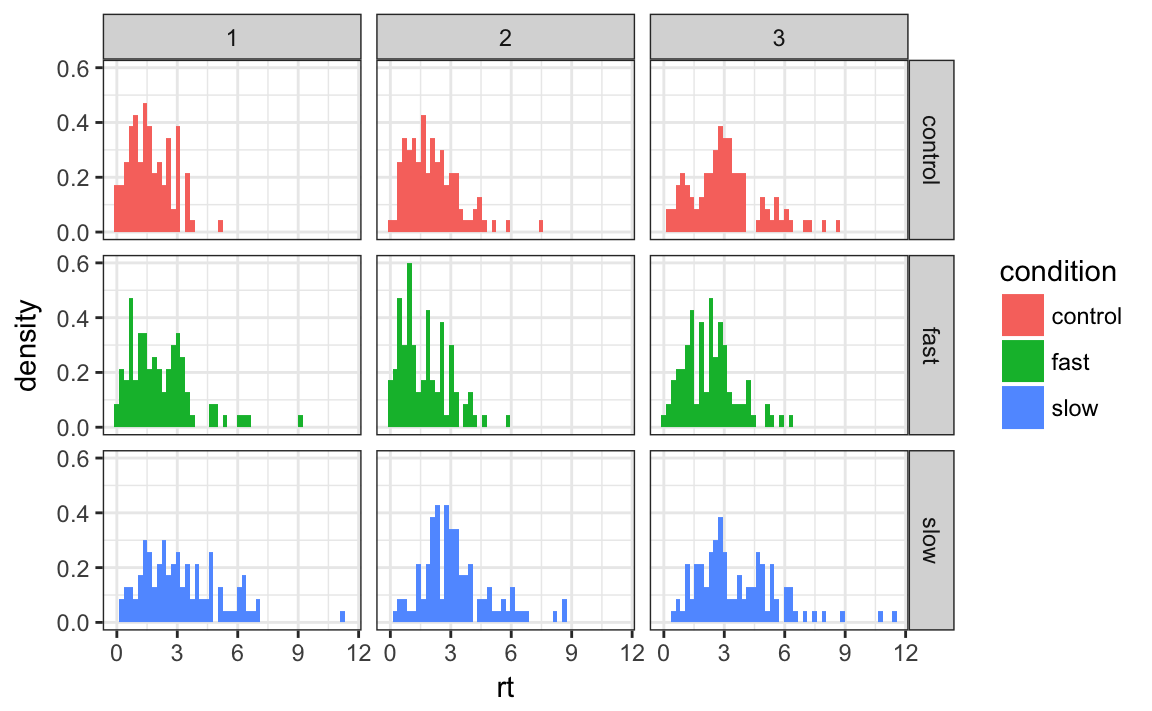

Adolescents in West and East Germany

library(dplyr)
library(tidyr)
library(stringr)
library(haven)

westost <- read_sav("data/Beispieldatensatz.sav")
westost
#> # A tibble: 286 x 126
#>      ID westost geschlecht alter  T1_1  T1_2  T1_3  T1_4  T1_5  T1_6  T1_7
#>   <dbl> <dbl+l>  <dbl+lbl> <dbl> <dbl> <dbl> <dbl> <dbl> <dbl> <dbl> <dbl>
#> 1  2.00       0          0  14.0  4.00  6.00  4.00  4.00  6.00  5.00  5.00
#> 2 14.0        0          0  14.0  3.00  5.00  5.00  4.00  5.00  7.00  5.00
#> 3 15.0        0          0  14.0  4.00  3.00  5.00  4.00  6.00  7.00  1.00
#> 4 17.0        0          0  15.0  6.00  6.00  5.00  5.00  7.00  6.00  5.00
#> 5 18.0        0          0  14.0  5.00  3.00  4.00  5.00  5.00  5.00  5.00
#> 6 19.0        0          0  15.0  6.00  6.00  6.00  6.00  7.00  7.00  5.00
#> # ... with 280 more rows, and 115 more variables: T1_8 <dbl>, T1_9 <dbl>,
#> #   T1_10 <dbl>, T1_11 <dbl>, T1_12 <dbl>, T1_13 <dbl>, T1_14 <dbl>, T1_15
#> #   <dbl>, T1_16 <dbl>, T1_17 <dbl>, T1_18 <dbl>, T1_19 <dbl>, T1_20
#> #   <dbl>, T1_21 <dbl>, T1_22 <dbl>, T1_23 <dbl>, T1_24 <dbl>, T1_25
#> #   <dbl>, T1_26 <dbl>, T1_27 <dbl>, T1_28 <dbl>, T1_29 <dbl>, T1_30
#> #   <dbl>, T1_31 <dbl>, T1_32 <dbl>, T1_33 <dbl>, T1_34 <dbl>, T1_35
#> #   <dbl>, T1_36 <dbl>, T2_1 <dbl>, T2_2 <dbl>, T2_3 <dbl>, T2_4 <dbl>,
#> #   T2_5 <dbl>, T2_6 <dbl>, T3_1 <dbl>, T3_2 <dbl>, T3_3 <dbl>, T3_4
#> #   <dbl>, T3_5 <dbl>, T3_6 <dbl>, T4_1 <dbl>, T4_2 <dbl>, T4_3 <dbl>,
#> #   T4_4 <dbl>, T4_5 <dbl>, T4_6 <dbl>, T4_7 <dbl>, T4_8 <dbl>, T4_9
#> #   <dbl>, T4_10 <dbl>, T4_11 <dbl>, T5_1 <dbl>, T5_2 <dbl>, T5_3 <dbl>,
#> #   T5_4 <dbl>, T5_5 <dbl>, T5_6 <dbl>, T5_7 <dbl>, T5_8 <dbl>, T5_9
#> #   <dbl>, T5_10 <dbl>, T5_11 <dbl>, T6_1 <dbl>, T6_2 <dbl>, T6_3 <dbl>,
#> #   T6_4 <dbl>, T6_5 <dbl>, T6_6 <dbl>, T6_7 <dbl>, T6_8 <dbl>, T6_9
#> #   <dbl>, T6_10 <dbl>, T6_11 <dbl>, T7_1 <dbl>, T7_2 <dbl>, T7_3 <dbl>,
#> #   T7_4 <dbl>, T7_5 <dbl>, T7_6 <dbl>, T7_7 <dbl>, T7_8 <dbl>, T7_9
#> #   <dbl>, T7_10 <dbl>, T7_11 <dbl>, T7_12 <dbl>, SES <dbl+lbl>, Deutsch
#> #   <dbl+lbl>, Mathe <dbl+lbl>, Fremdspr <dbl+lbl>, Schnitt <dbl>,
#> #   bildung_vater <dbl+lbl>, bildung_mutter <dbl+lbl>, bildung_vater_b
#> #   <dbl+lbl>, bildung_mutter_b <dbl+lbl>, swk_akad <dbl>, swk_selbstreg
#> #   <dbl>, swk_durch <dbl>, swk_motselbst <dbl>, swk_sozharm <dbl>, ...

westost <- westost %>%
    mutate(westost = factor(westost),
           geschlecht = factor(geschlecht),
           ID = factor(ID))

Mean age

Compute the mean age and standard deviation for both sexes.

westost %>%
    group_by(geschlecht) %>%
    summarise(alter_mw = round(mean(alter), 1),
              alter_sd = round(sd(alter), 1))
#> # A tibble: 2 x 3
#>   geschlecht alter_mw alter_sd
#>   <fct>         <dbl>    <dbl>
#> 1 0              14.8    0.700
#> 2 1              14.6    0.800

Emotional support

Select the variables unt_freunde (emotional support from friends) and unt_eltern (emotional support from parents) and use these to create a long data frame.

Step 1:

# select variables
unterstuetzung <- westost %>%
    select(ID, westost, unt_freunde, unt_eltern)

Step 2:

# handle missing values: are there any?
unterstuetzung[!complete.cases(unterstuetzung), ]
#> # A tibble: 2 x 4
#>   ID    westost unt_freunde unt_eltern
#>   <fct> <fct>         <dbl>      <dbl>
#> 1 332   1              4.83      NA   
#> 2 16    0             NA          5.17

# exclude missing values
unterstuetzung <- unterstuetzung %>%
    drop_na()

Step 3:

# convert wide to long
unterstuetzung <- unterstuetzung %>%
    gather(key = freunde_eltern,
           value = unterstuetzung, -ID, -westost)

Step 4:

# convert freunde_eltern variable to a factor
unterstuetzung <- unterstuetzung %>%
    mutate(freunde_eltern = factor(freunde_eltern))

Step 5 (advanced):

# rename factor levels (remove "unt_" prefix)
unterstuetzung <- unterstuetzung %>%
        mutate(freunde_eltern = str_replace(freunde_eltern, ".*_", ""))

Step 6:

# inspect resulting data frame
unterstuetzung
#> # A tibble: 568 x 4
#>   ID    westost freunde_eltern unterstuetzung
#>   <fct> <fct>   <chr>                   <dbl>
#> 1 2     0       freunde                  4.83
#> 2 14    0       freunde                  6.33
#> 3 15    0       freunde                  5.00
#> 4 17    0       freunde                  7.00
#> 5 18    0       freunde                  5.00
#> 6 19    0       freunde                  6.00
#> # ... with 562 more rows

And now all in one go:

unterstuetzung <- westost %>%
    select(ID, westost, unt_freunde, unt_eltern) %>%
    # fehlende Werte ausschliessen
    drop_na() %>%
    # von wide zu long
    gather(key = freunde_eltern,
           value = unterstuetzung, -ID, -westost) %>%
    # freunde_eltern variable bearbeiten
    mutate(freunde_eltern = factor(str_replace(freunde_eltern,
                                               ".*_", "")))
unterstuetzung
#> # A tibble: 568 x 4
#>   ID    westost freunde_eltern unterstuetzung
#>   <fct> <fct>   <fct>                   <dbl>
#> 1 2     0       freunde                  4.83
#> 2 14    0       freunde                  6.33
#> 3 15    0       freunde                  5.00
#> 4 17    0       freunde                  7.00
#> 5 18    0       freunde                  5.00
#> 6 19    0       freunde                  6.00
#> # ... with 562 more rows

Life Satisfaction

We want to investigate satisfaction in various contexts. The relevant variables all begin with leben_. We want to select all of these (exluding leben_gesamt, which is already a summary).

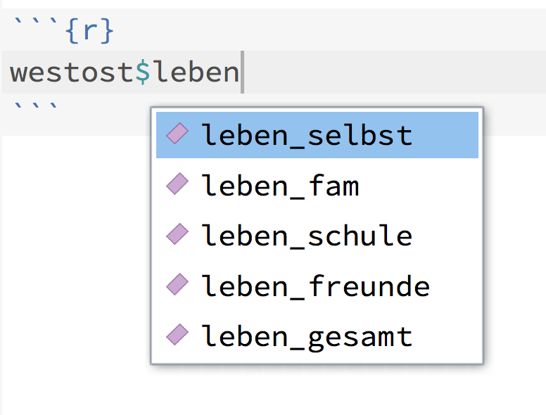We could choose all variables starting with leben_ using starts_with("leben_"), and then exclude leben_gesamt individually. We also want to retain each person ID.

zufriedenheit_wide <- westost %>%
    select(ID, starts_with("leben_"), -ends_with("gesamt"))
zufriedenheit_wide
#> # A tibble: 286 x 5
#>   ID    leben_selbst leben_fam leben_schule leben_freunde
#>   <fct>        <dbl>     <dbl>        <dbl>         <dbl>
#> 1 2             4.50      4.67         4.67          5.00
#> 2 14            5.00      5.33         5.00          6.00
#> 3 15            6.00      5.67         4.00          5.00
#> 4 17            6.00      6.00         5.00          6.00
#> 5 18            5.50      4.67         4.33          5.00
#> 6 19            6.00      6.67         4.00          6.50
#> # ... with 280 more rows

Can you think of any other ways of achieving this?

All selected variables can be considered as levels of an underlying (repeated-measures) factor. We can convert the data frame into a long format.

zufriedenheit_long <- zufriedenheit_wide %>%
    gather(key = lebensbereich, value = zufriedenheit, -ID)
#> Warning: attributes are not identical across measure variables;
#> they will be dropped

Now we need to consider what to do with missing values. Should we exclude all people with NAs in one context, or should we keep all observations?

First, we look for rows with NAs.

# head(20) displays the first 20 rows:
!complete.cases(zufriedenheit_wide) %>%
    head(20)
#>  [1] FALSE FALSE FALSE FALSE FALSE FALSE FALSE FALSE FALSE FALSE FALSE
#> [12] FALSE FALSE FALSE FALSE FALSE FALSE FALSE FALSE FALSE

This returns a logical vector, with either TRUE or FALSE for each row (it will be true if there is an NA in that row).

zufriedenheit_wide[!complete.cases(zufriedenheit_wide), ]
#> # A tibble: 2 x 5
#>   ID    leben_selbst leben_fam leben_schule leben_freunde
#>   <fct>        <dbl>     <dbl>        <dbl>         <dbl>
#> 1 175          NA           NA        NA            NA   
#> 2 206           5.00        NA         5.33          5.00

There are two participants with missing values - we decide to exlude these.

zufriedenheit_long <- zufriedenheit_wide %>%
    drop_na() %>%
    gather(key = lebensbereich, value = zufriedenheit, -ID)

The variable lebensbereich (context) should be converted into a factor:

zufriedenheit_long <- zufriedenheit_long %>%
    mutate(lebensbereich = as.factor(lebensbereich))
zufriedenheit_long
#> # A tibble: 1,136 x 3
#>   ID    lebensbereich zufriedenheit
#>   <fct> <fct>                 <dbl>
#> 1 2     leben_selbst           4.50
#> 2 14    leben_selbst           5.00
#> 3 15    leben_selbst           6.00
#> 4 17    leben_selbst           6.00
#> 5 18    leben_selbst           5.50
#> 6 19    leben_selbst           6.00
#> # ... with 1,130 more rows

We can also remove the prefix leben_ from each fator level.

library(stringr)
zufriedenheit_long <- zufriedenheit_long %>%
    mutate(lebensbereich = as.factor(str_replace(lebensbereich,
                                       ".*_", "")))

levels(zufriedenheit_long$lebensbereich)
#> [1] "fam"     "freunde" "schule"  "selbst"

Now we will sort by ID in ascending order:

zufriedenheit_long <- zufriedenheit_long %>%
    arrange(ID)
zufriedenheit_long
#> # A tibble: 1,136 x 3
#>   ID    lebensbereich zufriedenheit
#>   <fct> <fct>                 <dbl>
#> 1 1     selbst                 5.50
#> 2 1     fam                    7.00
#> 3 1     schule                 4.33
#> 4 1     freunde                6.50
#> 5 2     selbst                 4.50
#> 6 2     fam                    4.67
#> # ... with 1,130 more rows

All in one code chunk:

library(stringr) # for the str_replace() function

zufriedenheit_long <- zufriedenheit_wide %>%
    drop_na() %>%
    gather(key = lebensbereich, value = zufriedenheit, -ID) %>%
    mutate(lebensbereich = as.factor(str_replace(lebensbereich,
                                       ".*_", ""))) %>%
    arrange(ID)

Stress

Female adolescents are thought to be more prone to depressive disorders that male. We can use a t-test to test this hypothesis, but first we want to look at the data set and compute the mean and standard deviation for the variable stress_psych for each sex separately (rounded to 4 decimal places).

stress_psych <- westost %>%
    select(ID, geschlecht, stress_psych)
stress_psych
#> # A tibble: 286 x 3
#>   ID    geschlecht stress_psych
#>   <fct> <fct>             <dbl>
#> 1 2     0                  3.50
#> 2 14    0                  1.00
#> 3 15    0                  2.50
#> 4 17    0                  1.67
#> 5 18    0                  2.50
#> 6 19    0                  6.83
#> # ... with 280 more rows

stress_psych %>%
    group_by(geschlecht) %>%
    summarize(mean = mean(stress_psych),
              sd = sd(stress_psych))
#> # A tibble: 2 x 3
#>   geschlecht  mean    sd
#>   <fct>      <dbl> <dbl>
#> 1 0          NA    NA   
#> 2 1           3.10  1.12

There might be missing values. We have two options:

We remove all participants with NAs
We can leave all participants in the data set and handle any NAs using the na.rm argument in the mean() and sd() functions.

decimal_places <- 4

stress_psych %>%
    drop_na() %>%
    group_by(geschlecht) %>%
    summarize(mean = mean(stress_psych),
              sd = sd(stress_psych)) %>%
    mutate(mean = round(mean, decimal_places),
           sd = round(sd, decimal_places))
#> # A tibble: 2 x 3
#>   geschlecht  mean    sd
#>   <fct>      <dbl> <dbl>
#> 1 0           2.89  1.25
#> 2 1           3.10  1.12

stress_psych_summary <- stress_psych %>%
    group_by(geschlecht) %>%
    summarize(mean = mean(stress_psych, na.rm = TRUE),
              sd = sd(stress_psych, na.rm = TRUE)) %>%
    mutate(mean = round(mean, decimal_places),
           sd = round(sd, decimal_places))

stress_psych_summary
#> # A tibble: 2 x 3
#>   geschlecht  mean    sd
#>   <fct>      <dbl> <dbl>
#> 1 0           2.89  1.25
#> 2 1           3.10  1.12

library(ggplot2)

stress_psych %>%
    drop_na() %>%
    ggplot(aes(x = geschlecht, y = stress_psych, fill = geschlecht)) +
    geom_boxplot()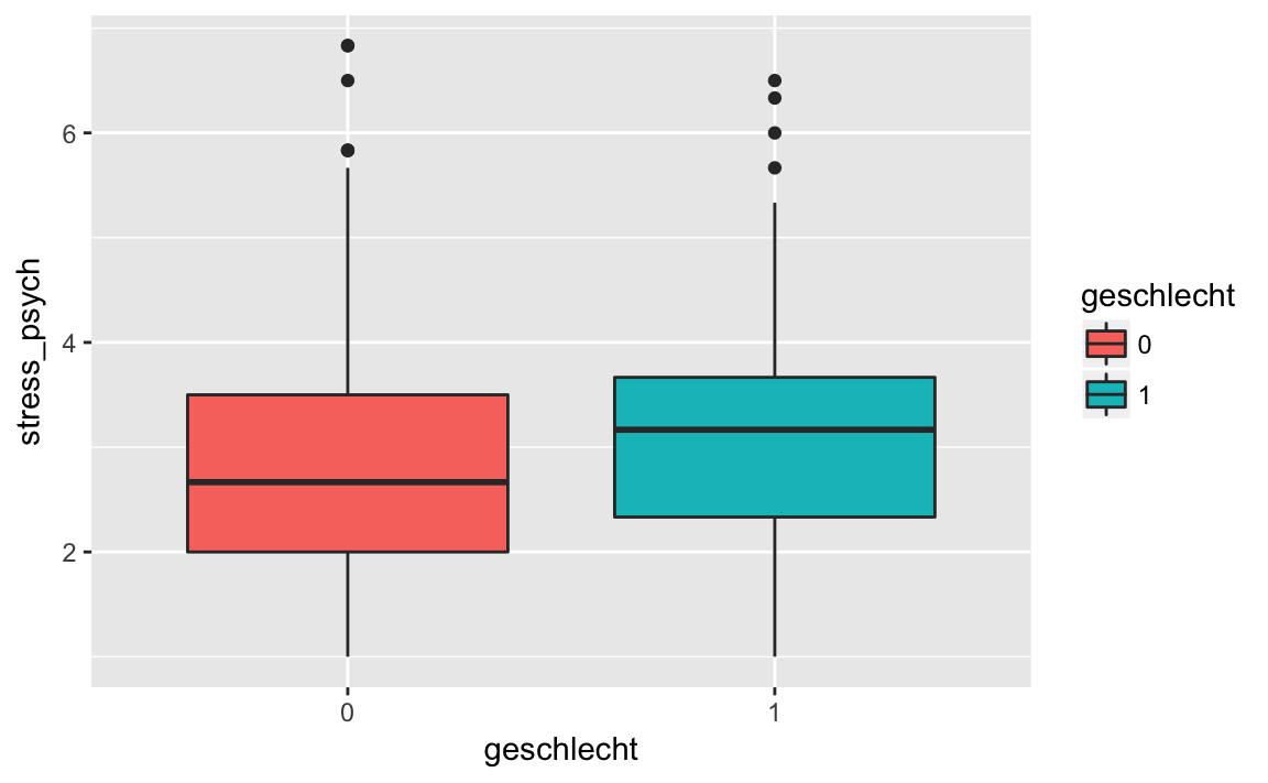

Job satisfaction: Honeymoon or hangover?

As a final example, we will investigate job satisfaction in people starting a new job. The hypothesis is that job satisfaction is U-shaped. In the beginning, job satisfaction is high (honeymoon), after a while, frustration kicks in (hangover). Eventually, job satisfaction rises again to a normal level.

Job satisfaction was measured in two companies at three time points: at the beginning, after three months and after six months.

Download and import the honeymoon.csv data set from von ILIAS. Pay attention to the delimiters used in the text file.

library(readr)
honeymoon <- read_delim("data/honeymoon.csv",
                        delim = ";")
#> Parsed with column specification:
#> cols(
#>   Firma = col_integer(),
#>   Anfang = col_integer(),
#>   Drei_Monate = col_integer(),
#>   Sechs_Monate = col_integer()
#> )

honeymoon
#> # A tibble: 10 x 4
#>   Firma Anfang Drei_Monate Sechs_Monate
#>   <int>  <int>       <int>        <int>
#> 1     1      9           4            5
#> 2     1      9           4            8
#> 3     1      9           7           14
#> 4     1     10           9            5
#> 5     1      8           1            3
#> 6     2     10          10           10
#> # ... with 4 more rows

The Firma variable should be a factor.

honeymoon <- honeymoon %>% mutate(Firma = as.factor(Firma))

Now we need a long data frame with a repeated measures factor Messzeitpunkt and a measured variable Arbeitszufriedenheit.

We will compute the mean job satisfaction for each person over all time points, the mean job satisfaction at each time points, seprately for each company.

First we need an ID variable. There are five employees in each company:

# nrow(.) means nrow(honeymoon) [place holder]
honeymoon <- honeymoon %>%
    mutate(ID = 1:nrow(.))

honeymoon_long <- honeymoon %>%
    gather(key = Messzeitpunkt, value = Arbeitszufriedenheit,
           -Firma, -ID) %>%
    mutate(Messzeitpunkt = factor(Messzeitpunkt))

levels(honeymoon_long$Messzeitpunkt)
#> [1] "Anfang"       "Drei_Monate"  "Sechs_Monate"

We can rename the factor levels from "Anfang", "Drei_Monate", "Sechs_Monate" to "0", "3", "6".

honeymoon_long <- honeymoon_long %>%
    mutate(Messzeitpunkt = recode_factor(Messzeitpunkt,
                           Anfang = "0",
                           Drei_Monate = "3",
                           Sechs_Monate = "6"))

honeymoon_long
#> # A tibble: 30 x 4
#>   Firma    ID Messzeitpunkt Arbeitszufriedenheit
#>   <fct> <int> <fct>                        <int>
#> 1 1         1 0                                9
#> 2 1         2 0                                9
#> 3 1         3 0                                9
#> 4 1         4 0                               10
#> 5 1         5 0                                8
#> 6 2         6 0                               10
#> # ... with 24 more rows

Next, we will sort by company and ID

honeymoon_long <- honeymoon_long %>%
    # Firma first, then ID
    arrange(Firma, ID)
honeymoon_long
#> # A tibble: 30 x 4
#>   Firma    ID Messzeitpunkt Arbeitszufriedenheit
#>   <fct> <int> <fct>                        <int>
#> 1 1         1 0                                9
#> 2 1         1 3                                4
#> 3 1         1 6                                5
#> 4 1         2 0                                9
#> 5 1         2 3                                4
#> 6 1         2 6                                8
#> # ... with 24 more rows

Now we can compute the mean job satisfaction for each person, for both companies separately. We can group by Firma and ID, and then compute the mean of the variable Arbeitszufriedenheit. We will add this new variable to the data frame honeymoon_long.

honeymoon_long <- honeymoon_long %>%
    group_by(Firma, ID) %>%
    mutate(Personenmittelwert = mean(Arbeitszufriedenheit))

honeymoon_long
#> # A tibble: 30 x 5
#> # Groups: Firma, ID [10]
#>   Firma    ID Messzeitpunkt Arbeitszufriedenheit Personenmittelwert
#>   <fct> <int> <fct>                        <int>              <dbl>
#> 1 1         1 0                                9               6.00
#> 2 1         1 3                                4               6.00
#> 3 1         1 6                                5               6.00
#> 4 1         2 0                                9               7.00
#> 5 1         2 3                                4               7.00
#> 6 1         2 6                                8               7.00
#> # ... with 24 more rows

Next, we want the mean for each time point, again for each company separately. We group by Firma and Messzeitpunkt.

honeymoon_long_bedingung <-
    honeymoon_long %>%
    group_by(Firma, Messzeitpunkt) %>%
    summarise(Bedingungsmittelwert = mean(Arbeitszufriedenheit))

honeymoon_long_bedingung
#> # A tibble: 6 x 3
#> # Groups: Firma [?]
#>   Firma Messzeitpunkt Bedingungsmittelwert
#>   <fct> <fct>                        <dbl>
#> 1 1     0                             9.00
#> 2 1     3                             5.00
#> 3 1     6                             7.00
#> 4 2     0                            10.0 
#> 5 2     3                            10.8 
#> 6 2     6                            11.0

honeymoon_long_bedingung %>%
    ggplot(aes(x = Messzeitpunkt,
               y = Bedingungsmittelwert,
               color = Firma,
               group = Firma,
               linetype = Firma)) +
    geom_point(size = 4) +
    geom_line(size = 2) +
    labs(x = "Messzeitpunkt (Monate)",
         y = "Arbeitszufriedenheit",
         title = "Honeymoon or Hangover?") +
    theme_classic()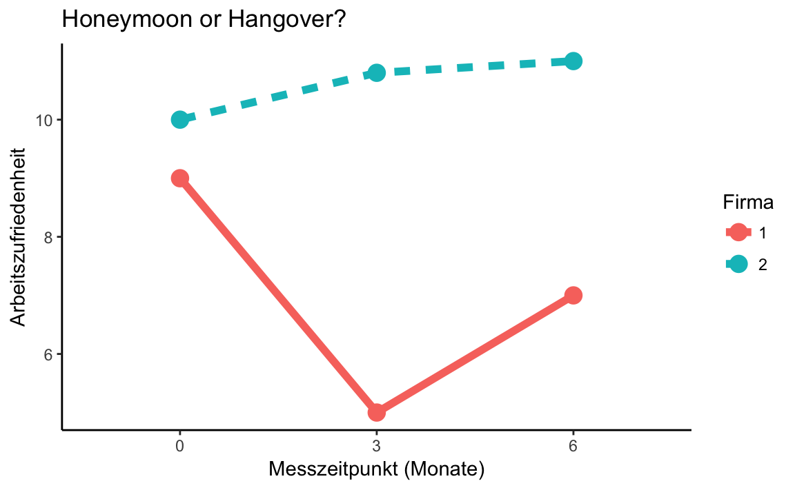

Really advanced: We have used the function str_replace() from the stringr package to rename factor levels. This function replaces strings and takes the arguments str_replace(string, pattern, replacement). string is the object in which to replace text, pattern is the text to be replaced (regular expression) and replacement is the replacement text.

In this example we want to replace the prefix leben_ by “” (empty string, or nothing). “.*_“ means: look for any character (.), repeated n times (*), followed by an underscore _.

str_replace("leben_freunde", ".*_", "")
#> [1] "freunde"

4 Working with Data

4.1 Tidy data

4.2 The pipe operator

Pipe syntax

4.3 Reshaping: tidyr

4.3.1 gather()

Example

4.3.2 spread()

Example

4.3.3 Excluding missing values (NAs): drop_na()

4.4 Data manipulation: dplyr

4.4.1 Selecting variables: select()

Examples

Changing the order of variables

“Helper” functions for select()

4.4.2 Renaming variables: rename()

Example

4.4.3 Selecting observations (cases): filter()

Examples

4.4.4 Sorting data frames: arrange()

4.4.5 Creating new variables: mutate()

Examples

4.4.6 Grouping data frames: group_by()

Examples

4.4.7 Recoding values: recode()

4.4.8 Summarizing variables: summarize()

Beispiele

4.4.9 Summary

4.5 Exercises

Reaction times

Adolescents in West and East Germany

Mean age

Emotional support

Life Satisfaction

Stress

Job satisfaction: Honeymoon or hangover?

4.3 Reshaping: `tidyr`

4.3.1 `gather()`

4.3.2 `spread()`

4.3.3 Excluding missing values (NAs): `drop_na()`

4.4 Data manipulation: `dplyr`

4.4.1 Selecting variables: `select()`

“Helper” functions for `select()`

4.4.2 Renaming variables: `rename()`

4.4.3 Selecting observations (cases): `filter()`

4.4.4 Sorting data frames: `arrange()`

4.4.5 Creating new variables: `mutate()`

4.4.6 Grouping data frames: `group_by()`

4.4.7 Recoding values: `recode()`

4.4.8 Summarizing variables: `summarize()`