1 RStudio Workflow
1.1 Graphical user interface (GUI)
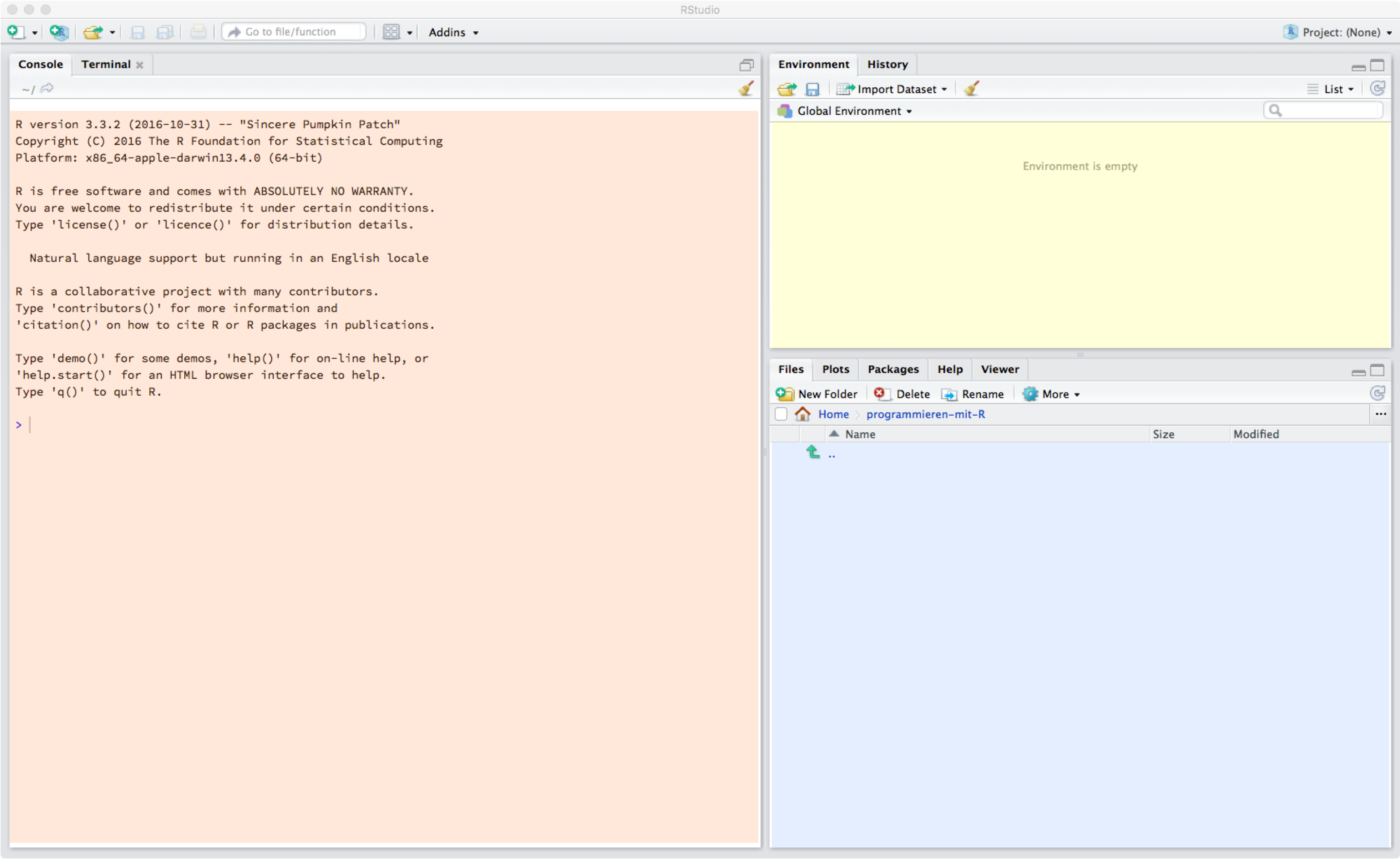
Let’s begin by exploring RStudio. When you open the program, it should look something like this:
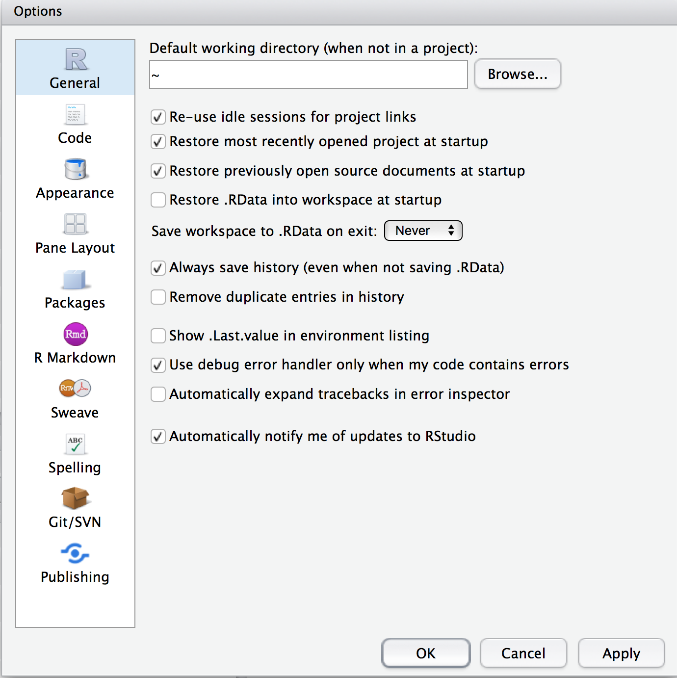
Under the Preferences or Global Options menu items, you can customize RStudio. We recommend not using the following options:
- Restore .RData into workspace at startup (Do not activate this)
- Save workspace to .RData on exit (Never) (Do not activate this)
It’s best to start each session with an empty workspace.
THe RStudio GUI is composed of several panes. On the left is the R console. This is where you can directly interact with R. If you enter a command here, and press Enter, the command will be interpreted by R.
The > symbol is called the R prompt. You can try to use R as a calulator:
2 + 3
#> [1] 5
exp(1)
#> [1] 2.72
3/4
#> [1] 0.75Top right (yellow): here, we have two panes Environment and History. In the Environment pane RStudio shows us all variables, datasets and functions that are available in the current session. If you click on the Global Environment drop-down menu, you can see which packages have been loaded.
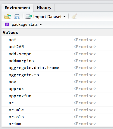
THe History pane shows a history of all commands that we have entered.
Bottom right (blue): here, we have the Files (file manager), Plots, Packages and Help Viewer panes.
Using the file manager, you can switch working directories and open files:
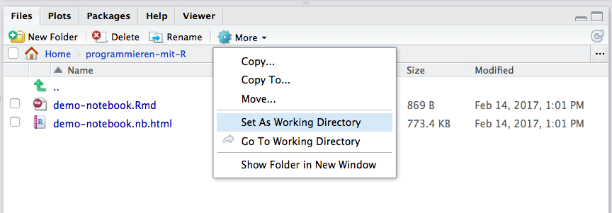
If you change working directories using the file manager, R will display the command in the console. In this case, the R command is setwd(…). By entering getwd(), you can ask R which directory you are currently in.
1.2 Packages
Before we start, we need to install some packages. Packages provide functionality that is not available in base R. We will need packages for manipulating data (tidyr, dplyr), for importing SPSS files (haven) and for plotting (ggplot2).
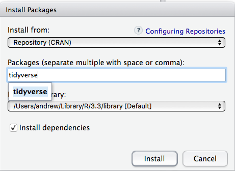
We can install all of these with the meta-package tidyverse using the command:
install.packages("tidyverse")Installed packages can be loaded using the library command:
library(tidyverse)We can also use the GUI:
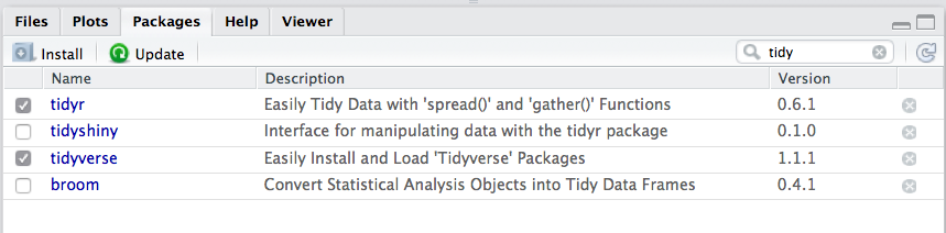
It’s a good idea to keep all paackages up to date. You can use (Update) in the Packages pane.
Please install the tidyverse packages.
R Packages are hosted on a server: The Comprehensive R Archive Network, or CRAN. Have a look at Task Views; these show a collection of packages for various topics, e.g. psychometrics CRAN Task View: Psychometric Models and Methods.
1.3 Help
In case you ever get stuck, RStudio has a built-in Help viewer:
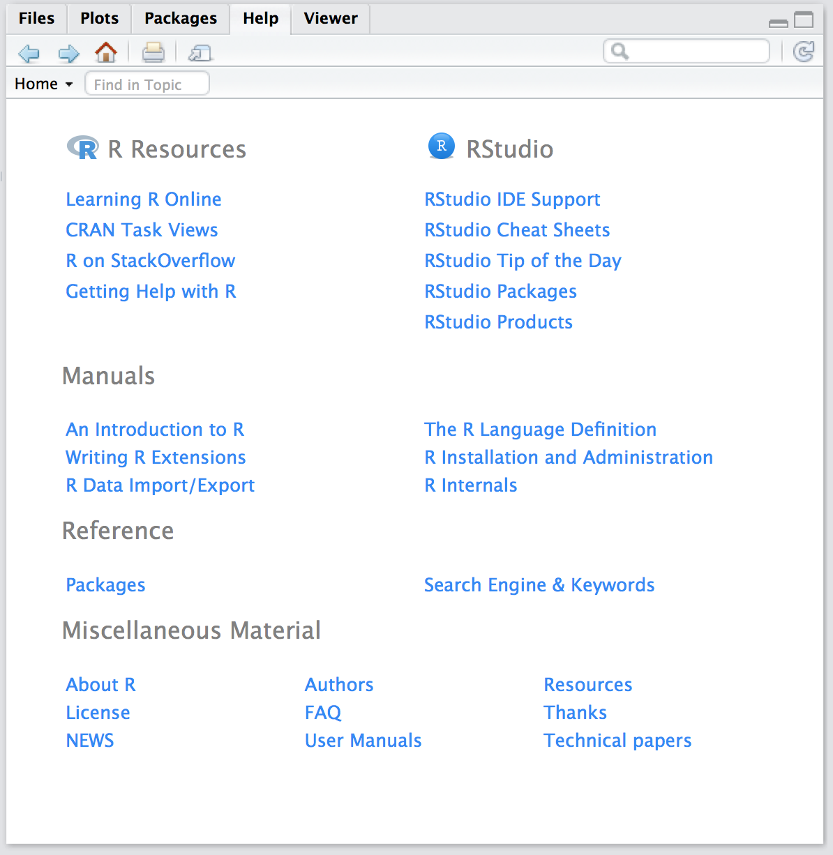
You can either enter a search term in the Help Viewers, or you can browse the packages to access their help pages.
Look for the package dplyr and click on it. You will a link to User guides, package vignettes and other documentation. Vignettes are introductory manuals.
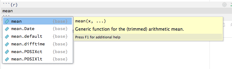
You can also access help directly in the console:
help(mean)This will open the help page for the mean function. You can also enter?mean.
We also often use the Q & A website Stackoverflow - here you can find an answer to just about any question.
1.4 Working with RStudio
1.4.1 Projects
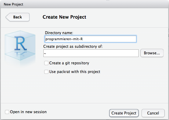
We recommend using an RStudio project. Go to File > New Project. You can give your project a name.
1.4.2 Console
You can either enter commands directly into the console, or write in a text file, and then send the command to the console.
Working in the console is ok for quickly trying things out, but usually it is better to use text files.
You can access your History in the console using the CMD + Up or CTRL + Up keys. You can access your latest commands in the console using the Up key (several times for earlier commands). Once you used the Up key (several times) you can use the Down key to access later commands. This is useful when you want to do something again or do something very similar by adjusting earlier commands.
If you forget to complete an R command, you might see this:
> mean(x
+
This means that R is waiting for you to complete your command. In this case, you can either enter ) or press ESCAPE. With ) you correctly finish the command, with ESCAPE you get a new prompt and can start over.
1.4.3 R Script
Let’s open an R script (text file with the file ending .R). Enter the R code:
2 + 3
#> [1] 5
Then you can select the code, and click on Run. You will see the output in the console.
Enter and run the following code: x <- c(101, 105, 99, 87, 102, 98)
You just defined a vector (or a variable). You will see the following in the output:
> x <- c(101, 105, 99, 87, 102, 98)
and in the Environment you will see that x is a num [1:6]. This means that x is a numeric vector with length 6, i.e. consisting of 6 elements.
Try running: boxplot(x)
You should see a box plot in the Plots pane.
1.4.4 Using R Notebooks
R Notebooks are interactive RMarkdown documents (RMarkdown is a simple markup language). These can display text, code and graphics, all in the same document.
Open a new notebook file: 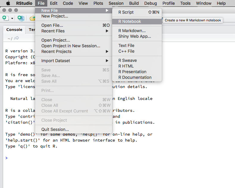
You can save the notebook with the file ending .Rmd.
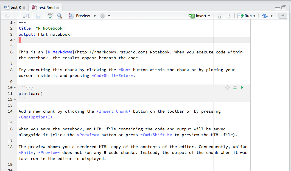
Notebooks contain both Markdown text and code chunks. These code chunks can be evaluated.
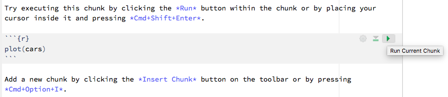
When you press the green arrow the output will appear right beneath the code chunk.
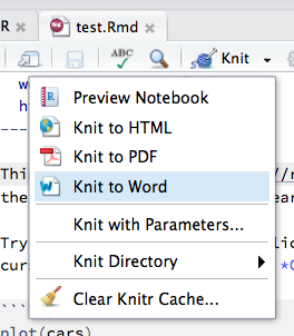
The whole document can be compiled by clicking on Preview. THe first time you do this, RStudio will ask you to install some missing packages (you should do this). After compilation, you will see an HTML document in the Viewer pane. You can also create Word documents or PDFs:
1.4.5 Tab completion
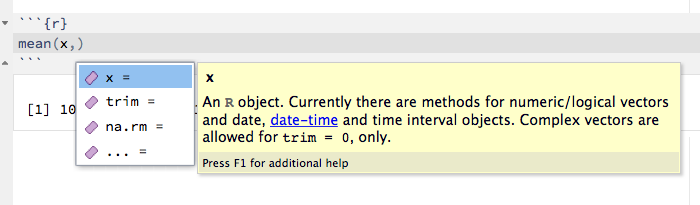
RStudio has a very useful feature: tab completion. If you enter R commands in the console or in the text editor, R will automatically provide you with a list of possible completions. We can also get suggestions, including possible arguments of functions, by pressing the tab key.
We can also use this feature to look for functions inside packages. For example, we can write a package name, followed by :: and the press tab. RStudio will give us a list of functions from that package. To get a list of all functions starting with the letter f from the dplyr package:
dplyr::f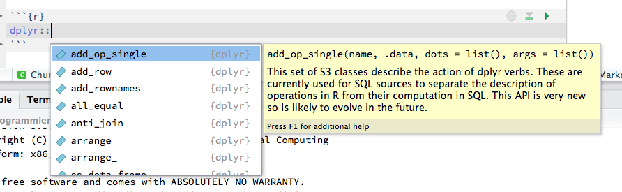
1.4.6 Key combinations
We will need the following symbols:
[ ]  Square braces
{ }  Curly braces
$    Dollar key
#    Hash (pound) key
~    Tilde (for formula notation)
|    Vertical bar
`    Backtick
Unfortunately, these can be somewhat difficult to find on German/Swiss keyboards.
Take a few minutes to familiarize yourself with your keyboard. You will need to use the ALT key for some of the symbols.
We entered
3/4, and we got[1] 0.75as output. This means that the output starts with the first element of a vector.