6 Statistical Distributions

R provides a very simple and effective way of calculating distribution characteristics for a number of distributions (we only present part of it here).

An overview of all available distributions is can be found via help(“Distributions”).

6.1 Normal distribution

We will introduce the different statistical functions using the normal distribution and then look at other distributions. With help("Normal") we get an overview of the statistical functions for the normal distribution:

dnorm(x, mean = 0, sd = 1,      # Probability density function 
      log = FALSE)                       
pnorm(q, mean = 0, sd = 1,      # Cumulative distribution function (computing 
      lower.tail = TRUE,        # tail probabilities for z scores)
      log.p = FALSE)  
qnorm(p, mean = 0, sd = 1,      # Quantile function (computing z scores for probabilities)
      lower.tail = TRUE,        # -> Inverse cumulative distribution function
      log.p = FALSE)  
rnorm(n, mean = 0, sd = 1)      # Pseudo-random number generator of normally distributed scores

Arguments

x, q   vector of quantiles.     # Normally distributed value(s), for which the probability density 
                                # [dnorm()] or the distribution function [pnorm()] will be computed.
p      vector of probabilities. # Cumulative probability or probabilities, for which 
                                # the quantile of a normal distribution will be computed 
n      number of observations.  # Number of random numbers to be generated with rnorm() 
mean   vector of means.         # Expected value(s) of one or more normal distributions
sd     vector of SDs.           # Standard deviation(s) of one or more normal distributions
log, log.p   logical;           # computes all statistics for lognormal distributions 
   are given as log(p).  
lower.tail   logical;           # if FALSE: 1) with pnorm() instead of the cumulative  
   if TRUE (default),           #  distribution function P[X ≤ x] the complementary 
                                # function P[X > x] will be computed;
   probabilities are P[X ≤ x]   # 2) when computing quantiles using qnorm() the argument
                                # p is interpreted as 1-p

Cumulative distribution function (CDF)

The distribution function pnorm() is needed to calculate p-values. The simplest case concerns the left tail (one-tailed) p-value for a given standard-normally distributed empirical z score.

If we do not specify the arguments mean and sd, the default values mean = 0 and sd = 1 are used and we get the standard normal distribution.

Example:

pnorm(q = -1.73)
#> [1] 0.04181514

# or simply

pnorm(-1.73)
#> [1] 0.04181514

The p-value for a one-tailed (left-tailed) significance test for z = -1.73 is 0.042.

If we need a right-tailed p-value (area to the right of a certain empirical z-score) we use the argument lower.tail = FALSE.

pnorm(1.645)  # this is 1-p
#> [1] 0.9500151
pnorm(1.645, lower.tail = FALSE)
#> [1] 0.04998491

The value of 1.645 of the standard normal distribution is often used as a critical value for the one-tailed significance test. So to left of this value should be 95% of the distribution and to the right of it 5% of the distribution. Here we see that this is not exactly true.

For a two-tailed p-value we’ll have to double the one-tailed p-value:

# 2-tailed p-value for a negative z-score
2*pnorm(-1.73)
#> [1] 0.08363028

# 2-tailed p-value for a negative z-score
2*pnorm(1.73, lower.tail = FALSE)
#> [1] 0.08363028
2*(1 - pnorm(1.73))
#> [1] 0.08363028

We can also use pnorm() to get the percentiles of a series of normally distributed values. For example, we want to know which percentiles correspond to a set of IQ values:

IQ_Scores <- c(74, 87, 100, 110, 128, 142)
pnorm(q = IQ_Scores, mean = 100, sd = 15)
#> [1] 0.04151822 0.19306234 0.50000000 0.74750746 0.96902592 0.99744487

The IQ scores 74, 87, 100, 110, 128, 142 thus correspond to the percentiles 4.2%, 19.3%, 50%, 74.8%, 96.9%, 99.7% of the IQ distribution.

It is also possible to compute the probability of any interval between two normally distributed scores by subtracting the two respective cumulative distribution functions.

# Probability of z-scores between -0.5 and + 0.5
pnorm(0.5) - pnorm(-0.5)
#> [1] 0.3829249

# Probability of IQ-scores between 130 and 140
pnorm(140, mean = 100, sd = 15) - pnorm(130, mean = 100, sd = 15)
#> [1] 0.01891975

Quantile function

The quantile function qnorm() is the complement to the distribution function. It is also called inverse cumulative distribution function (ICDF). With qnorm() we obtain a z-score (i.e., a quantile of the standard normal distribution) for a given area p representing the first argument of the function. In practice, we often need this function to calculate critical values for a given \(\alpha\)-level for one-tailed and two-tailed significance tests.

The most frequently used z quantiles for \(\alpha\) = 0.01 and \(\alpha\) = 0.05 are:

# alpha = 0.01
qnorm(p = 0.005)    # two-tailed test, lower critical value
#> [1] -2.575829
qnorm(p = 0.995)    # two-tailed test, upper critical value 
#> [1] 2.575829
qnorm(p = 0.01)     # one-tailed test, left critical value
#> [1] -2.326348
qnorm(p = 0.99)     # one-tailed test, right critical value
#> [1] 2.326348
                                       
# alpha = 0.05
qnorm(p = 0.025)    # two-tailed test, lower critical value
#> [1] -1.959964
qnorm(p = 0.975)    # two-tailed test, upper critical value
#> [1] 1.959964
qnorm(p = 0.05)     # one-tailed test, left critical value
#> [1] -1.644854
qnorm(p = 0.95)     # one-tailed test, right critical value
#> [1] 1.644854

Alternatively, the upper or right-tailed critical values can be computed with the lower quantile and the argument lower.tail = FALSE: qnorm (p = 0.975) is equivalent to qnorm (p = 0.025, lower.tail = FALSE )

We can use the quantile function also more generally, e.g., for the deciles of the IQ distribution:

deciles <- seq(0, 1, by = 0.1)
qnorm(p = deciles, mean = 100, sd = 15)
#>  [1]      -Inf  80.77673  87.37568  92.13399  96.19979 100.00000 103.80021
#>  [8] 107.86601 112.62432 119.22327       Inf

With an IQ of just under 120, you thus belong to the smartest 10% of the population!

Probability density function (PDF)

We actually rarely need the probability density function (PDF) of a normally distributed score. As a reminder: the probability of individual values of a continuous random variable is 0, only intervals of values have a probability greater than 0 (corresponding to the area under the curve, the integral). Individual values have a probability density, which corresponds to the height of the curve of the probability distribution at the point X = x. Thus, we need the probability density function if we want to plot a normal distribution.

Before we start plotting, let’s have a look at the definition of the probability density function of the standard normal distribution: \(\phi(z) = \frac{1}{\sqrt{2\cdot\pi\cdot e^{z^{2}}}}\). The density for the mean (\(\mu\) = 0) is therefore \(\phi(z) = \frac{1}{\sqrt{2\cdot\pi\cdot e^{0^{2}}}} = \frac{1}{\sqrt{2\cdot\pi}}\):

1/(sqrt(2*pi))
#> [1] 0.3989423

# and that is:

dnorm(x = 0)
#> [1] 0.3989423

We then get the probability density function for z = 1 as:\(\phi(z) = \frac{1}{\sqrt{2\cdot\pi\cdot e^{1^{2}}}} = \frac{1}{\sqrt{2\cdot\pi\cdot e}}\):

1/(sqrt(2*pi*exp(1)))
#> [1] 0.2419707

# or as:

dnorm(1)
#> [1] 0.2419707

Plotting the standard normal distribution

library(tidyverse)
p <- data_frame(x = c(-4,4)) %>% 
    ggplot(aes(x = x)) 
#> Warning: `data_frame()` is deprecated, use `tibble()`.
#> This warning is displayed once per session.

p + geom_vline(xintercept = 0, linetype = "dashed", alpha = 0.4) +
    stat_function(fun = dnorm, color = "#84CA72", size = 1.5) +
    ggtitle("Standard Normal Distribution") +
    xlab("x") +
    ylab("dnorm(x)") +
    theme_classic()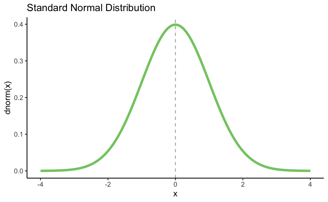

We can also draw a certain z score in the diagram and let us calculate a p-value for this with pnorm():

my_z <- 1.73

p_value <- round(pnorm(my_z, lower.tail = FALSE), 3)

p + geom_segment(aes(x = my_z, 
                     y = 0, 
                     xend = my_z, 
                     yend = (dnorm(my_z))), 
                 color = "grey70", 
                 size = 1.5, 
                 alpha = 0.8) +
    stat_function(fun = dnorm, color = "#84CA72", size = 1.5) +
    ggtitle("Standard Normal Distribution") +
    xlab("x") +
    ylab("dnorm(x)") +
    annotate("text", label = paste0("p = ", p_value), 
             x = my_z + 0.7, 
             y = 0.1, 
             color = "black") +
    theme_classic()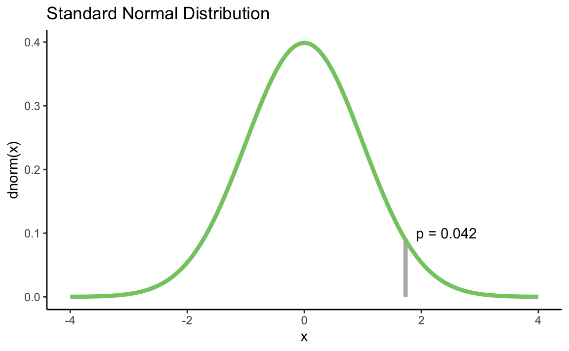

Data simulation

With rnorm() we can generate normally distributed pseudo-random numbers. It is a pseudo-random number generator because the function only simulates randomness. An actual random number generator is a bit complicated and can not be easily implemented using a deterministic computer. The advantage of the pseudo-random generator is that we can get a reproducible “random” draw using the seed value function. set.seed () starts the draw algorithm at a specific location, so that the same starting numbers always return the same “random” numbers.

Let’s generate 22 “random” IQ scores:

set.seed(534)  # or any other number
r_IQ_scores <- rnorm(n = 22, mean = 100, sd = 15)
r_IQ_scores
#>  [1]  91.85366 112.20598  93.59749  95.60904  89.71878  93.37631  87.61408
#>  [8]  92.83598  93.02380  88.35326 132.49322  87.30990 107.95051  95.45687
#> [15]  92.59292  84.40998 135.42350  67.04528  91.38498 130.92657  81.36571
#> [22] 102.44571
mean(r_IQ_scores)
#> [1] 97.59062
sd(r_IQ_scores)
#> [1] 16.91699

6.2 t distribution

With help("TDist") we obtain an overview of the functions for the t distribution:

dt(x, df, ncp               # Probability density function of the t distribution 
      log = FALSE)                   
pt(q, df, ncp,              # Cumulative distribution function (computing tail 
      lower.tail = TRUE,    # probabilities for t scores)
      log.p = FALSE)  
qt(p, df, ncp               # Quantile function (computing t scores for probabilities)
      lower.tail = TRUE,    # -> Inverse cumulative distribution function
      log.p = FALSE)  
rt(n, df, ncp)              # Pseudo-random number generator of t distributed scores            

The function arguments are the same as for the normal distribution with the following differences: The degrees of freedom (df) of the t distribution must be specified. The arguments mean and sd are omitted, but there is the non-centrality parameter ncp. This is needed (as the name suggests) for non-central t distributions that do not have a mean of 0. While the central t distribution (with \(\mu = 0\)) is symmetric and corresponds to the H0 distribution required for t tests, the non-central t distributions (H1 distributions) are asymmetric and required for power analysis. We will not look at these distributions here, so we will not use the ncp argument.

Cumulative distribution function (CDF)

Example for a one-tailed (left-tailed) p-value:

pt(q = -1.73, df = 6)
#> [1] 0.06717745
pt(-1.73, 6)
#> [1] 0.06717745

Example for a one-tailed (right-tailed) p-value

pt(1.73, df = 6, lower.tail = FALSE)
#> [1] 0.06717745

For a two-tailed significance test we would need to double the one-tailed p-value:

# 2-tailed p-value for a negative t
2 * pt(-1.73, df = 6)
#> [1] 0.1343549

# 2-tailed p-value for a positive t
2 * pt(1.73, df = 6, lower.tail = FALSE)
#> [1] 0.1343549

Quantile function

With qt() we get a t score for a given area p. In most t distribution tables, only specific t quantiles are tabulated. In the textbook by Eid, Gollwitzer & Schmitt (2015), e.g. the t scores for the distribution functions p of 0.6, 0.8, 0.9, 0.95, 0.975, 0.99 and 0.995 are given for t distributions with various degrees of freedom.

Let’s get these for a t-distribution with df = 6:

my_ps <- c(0.6, 0.8, 0.9, 0.95, 0.975, 0.99, 0.995)
qt(my_ps, df = 6)
#> [1] 0.2648345 0.9057033 1.4397557 1.9431803 2.4469119 3.1426684 3.7074280

Compare these t quantiles with those from the t table! Calculate additional quantiles for t distributions with df > 30 that are not available in the table. (You will never again have to approximate a critical t score with a z score because the table does not include the specific t distribution you need…)

Probability density function (PDF)

Let’s plot a t distribution:

library(tidyverse)
p <- data_frame(x = c(-4,4)) %>% 
    ggplot(aes(x = x)) 

p + stat_function(fun = dt, args = list(df = 6), color = "#84CA72", size = 1.5) +
    ggtitle("Central t-Distribution (df = 6)") +
    xlab("x") +
    ylab("dt(x, df = 6)") +
    theme_classic()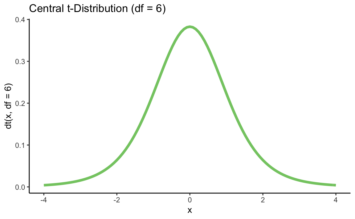

library(tidyverse)
p <- data_frame(x = c(-4,4)) %>% 
    ggplot(aes(x = x)) 

p + stat_function(fun = dt, args = list(df = 6), color = "#84CA72", size = 1.5) +
    stat_function(fun = dnorm, color = "grey70", size = 1.5) +
    ggtitle("Central t-Distribution (df = 6) compared to z-Distribution") +
    xlab("x") +
    ylab("dt(x, 6) / dnorm(x)") +
    theme_classic()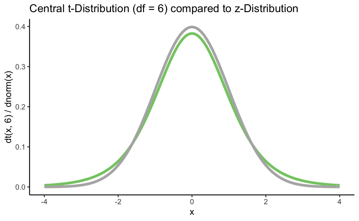

Data simulation

With rt() we can randomly generate t distributed scores. The functionality is the same as for the normal distribution.

6.3 Chi-square distribution

For the chi-square distribution (help ("chisquare")) the functionality is the same as for the t distribution. The respective degrees of freedom must be specified and there are also non-central distributions, which we will not consider further. The functions are called pchisq() (cumulative distribution function), qchisq() (quantile function), dchisq() (density function) and rchisq() (random generation of \(\chi^2\)-distributed scores).

Cumulative distribution function (CDF)

When calculating p-values for the chi-square distribution, in most cases only the upper (right) end of the distribution is needed. This is because most statistical tests are designed in such a way that all deviations from H0 (no matter in which direction) lead to a larger chi-square value (that’s why these tests always test a non-directional hypothesis, and the p-value therefore corresponds to a two-tailed test). Thus, we always use the argument lower.tail = FALSE to calculate p-values for chi-square distributions.

There are some exceptions: One is the chi-square test for comparing a sample variance to a known population variance (one-sample variance test). For this test in some cases the lower (left) end of chi-square distribution is needed. Since the chi-square one-sample variance test is not implemented in most statistical packages, one could actually be confronted with the need to compute such a p-value by hand (using pchisq() with the default value `lower.tail = TRUE)…

Example for a p-value for \(\chi^2(2) = 4.56\)

pchisq(q = 4.86, df = 2, lower.tail = FALSE)
#> [1] 0.08803683

Quantile function

With qchisq() we obtain the quantiles of the chi-square distribution, e.g. the critical values for \(\alpha = 0.05\). Some statisticians are very proud to know the critical values for the 1, 2, 3, 4, and 5 degrees of freedom of the chi-square distributions by heart, because these are often needed for model comparisons via likelihood ratio tests.

my_dfs <- 1:5
round(qchisq(0.95, df = my_dfs), 2)
#> [1]  3.84  5.99  7.81  9.49 11.07

Probability density function (PDF)

Again, we can use the probability density function dchisq() to plot one or more chi-square distributions:

library(tidyverse)
p <- data_frame(x = c(0, 25)) %>% 
    ggplot(aes(x = x)) 

p + stat_function(fun = dchisq, args = list(df = 2), color = "#84CA72", size = 1.5) +
    stat_function(fun = dchisq, args = list(df = 4), color = "grey70", size = 1.5) +
    stat_function(fun = dchisq, args = list(df = 8), color = "blue", size = 1.5, alpha = 0.7) +
    stat_function(fun = dchisq, args = list(df = 14), color = "red", size = 1.5, alpha = 0.7) +
    ggtitle("Chi-Square Distributions with dfs = 2, 4, 8, and 14") +
    xlab("x") +
    ylab("dchisq(x, c(2, 4, 8, 14))") +
    theme_classic()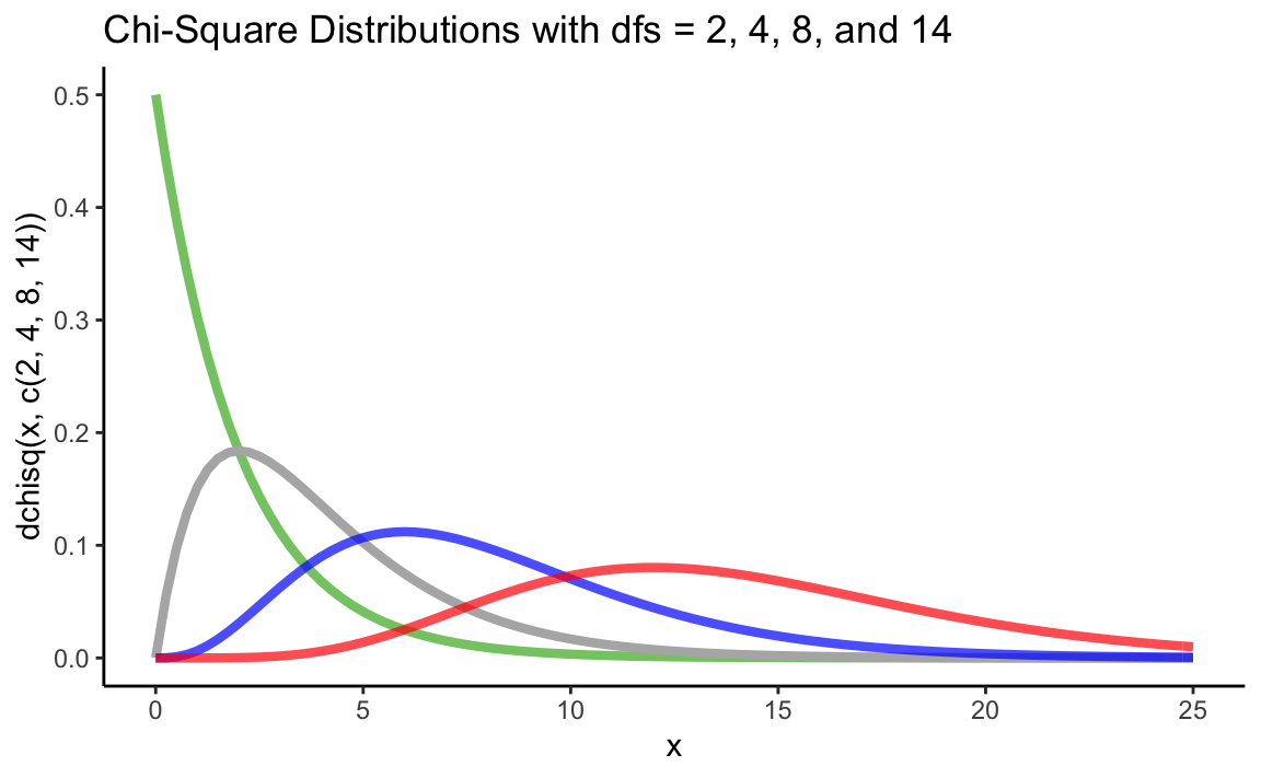

Data simulation

With rchisq() we can generate \(\chi^2\)-distributed random numbers. The functionality is the same as for the other distributions.

6.4 F distribution

For the F distribution (help ("FDist")), the same rules apply as for the \(\chi^2\)-distribution and for the t distribution. We have to specify both numerator degrees of freedom (df₁) and denominator degrees of freedom (df₂). The functions are pf() (cumulative distribution function),qf() (quantile function), df() (probability density function), and rf() (random generation of F distributed scores).

Cumulative Distribution Function

When calculating p-values for the F distribution, in most cases only the upper (right) end of the distribution is needed (as with the \(\chi^2\)-distribution). We therefore always use the argument lower.tail = FALSE to calculate p-values. Probably the most typical application for the F test is the one-factorial analysis of variance. Here we test whether there are any significant differences in the mean values between several groups. All deviations from H0 lead to a larger SSQ_between and thus to a higher empirical F-statistic. That’s also why we consider the entire \(\alpha\) at the upper end of the distribution when computing critical F scores (see below “Quantile Function”).

Example for a p-value for F = 3.89 (df₁ = 2, df₂ = 40):

pf(q = 3.89, df1 = 2, df2 = 40, lower.tail = FALSE)
#> [1] 0.02859413

Quantile function

If we compute an ANOVA by hand ;) often F distribution tables do not contain all combinations of degrees of freedoms. With qf() we can obtain the quantiles of the F distribution, thus the critical values for a significance test.

Example: Critical values for \(\alpha = 0.05\) and \(\alpha = 0.01\) for an F distribution with df₁ = 2 and df₂ = 40:

qf(c(0.95, 0.99), df1 = 2, df2 = 40)
#> [1] 3.231727 5.178508

# or also

qf(c(0.05, 0.01), df1 = 2, df2 = 40, lower.tail = FALSE)
#> [1] 3.231727 5.178508

Probability density function (PDF)

Let’s plot some F distributions using df():

library(tidyverse)
p <- data_frame(x = c(0, 5)) %>% 
    ggplot(aes(x = x)) 

p + stat_function(fun = df, args = list(df1 = 2, df2 = 40), 
                  color = "#84CA72", size = 1.5) +
    stat_function(fun = df, args = list(df1 = 5, df2 = 80), 
                  color = "grey70", size = 1.5) +
    stat_function(fun = df, args = list(df1 = 8, df2 = 120), 
                  color = "blue", size = 1.5, alpha = 0.7) +
    ggtitle("F-Distributions with df1 = 2, 5, 8 and df2 = 40, 80, 120") +
    xlab("x") +
    ylab("df(x, c(2, 5, 8), c(40, 80, 120))") +
    theme_classic()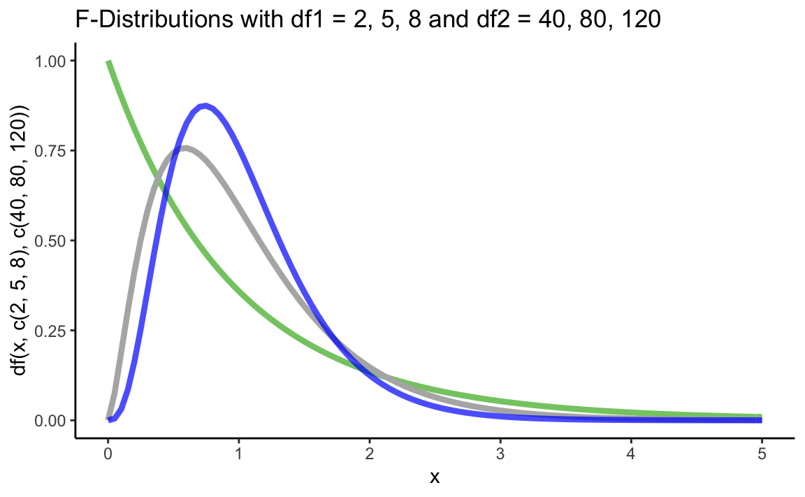

Data simulation

With rf() we can generate F distributed random numbers. The functionality is the same as for the other distributions.

6.5 Exercises

Densities and plots

Compute the probability densities of the following IQ-scores: 70, 80, 90, 100, 110, 120, 130

Plot the following two normal distributions into a common plot: \(N(\mu = 0,\sigma^{2} = 1)\) und \(N(\mu = 3,\sigma^{2} = 0.75)\). Use different colors for the two distributions. Hint: variance \(\neq\) SD!

library(tidyverse)
p <- data_frame(x = c(-4,7)) %>% 
    ggplot(aes(x = x)) 

p + stat_function(fun = dnorm, color = "#84CA72", size = 1.5) +
    stat_function(fun = dnorm, args = list(3, sqrt(0.75)), color = "purple", size = 1.5, alpha = 0.6) +
    ggtitle("2 Normal Distributions") +
    xlab("x")+
    ylab("dnorm(x)") +
    theme_classic()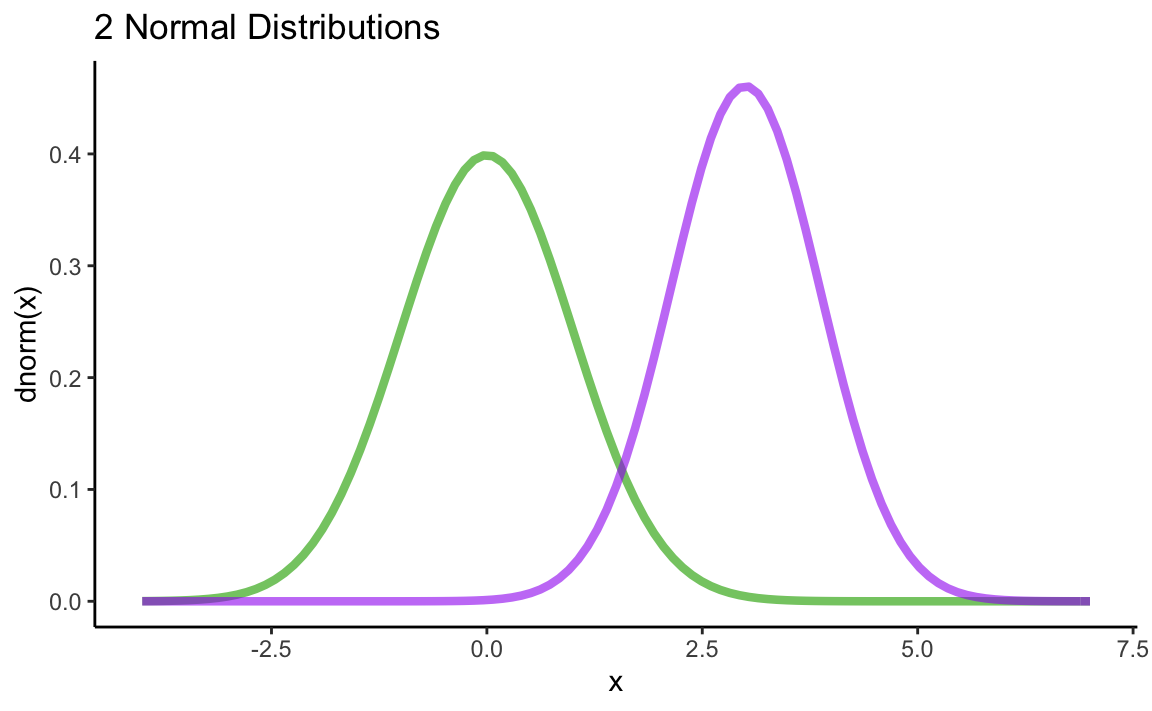

Cumulative distribution functions and p-values

Compute the cumulative distribution function for z = 1.

Compute the probability of values +/- 1 SD of the mean for any normal distribution (i.e. the area of this interval under the normal curve).

What is the percentange of the population that has IQs between 105 and 120?

Compute a one-tailed (right-tailed) p-value for a test statistic t= 2.045 (df = 8).

Compute a two-tailed p-value for a test statistic t= 0.73 (df = 14)

Compute a two-tailed p-value for a test statistic t= -0.73 (df = 14)

You got a test statistic of F= 4.36. Is the test significant (df₁ = 2, df₂ = 16)?

Quantiles and critical values

Sixty percent of the population are below or equal to which IQ-score? Calculate the 60%-quantile of the IQ distribution.

Five percent of the population are above or equal to which IQ-score?

Advanced: Between which two IQ scores lie the middle 82% of the population? (We are looking for the 82%- Central Probability Interval)

Calculate the critical t-score (df = 28) for a one-tailed (right-tailed) test with \(\alpha = 0.05\).

Calculate the critical t-scores (df = 28) for a two-tailed test with \(\alpha = 0.05\).

Calculate the critical F-score for df₁ = 5 and df₂ = 77 (\(\alpha = 0.01\)).