2 The R Language
2.1 Operators and functions
In order to use R as a calculator, we will need to master some basic vocabulary.
To start with, let’s look at some arithmetic and logical operators.
2.1.1 Arithmetic operators
The first five should be self-explanatory:
+                addition
-                subtraction
*                multiplication
/                division
^ or **          power

x %*% y          matrix multiplication c(5, 3) %*% c(2, 4) == 22
x %% y           modulo (x mod y) 5 %% 2 == 1
x %/% y          whole number division: 5 %/% 2 == 2
The last three operators may be new to you. %*% is the operator for [matrix multiplication] (https://en.wikipedia.org/wiki/Matrix_multiplication). %% ist der modulo operator. This finds the remainder after division, e.g. 5 %% 2 (5 modulo 2) is equal to 1. %/% is a whole number division, e.g. 5 %/% 2 is equal to 2 (how many times is 2 contained in 5?). These operators are often used for programming.
2.1.2 Logical operators and functions
You probably won’t need the last two functions, xor() and isTRUE() very often.
<                less than
<=               less than or equal to
>                greater than
>=               greater than or equal to
==               equal
!=               not equal
!x               not x (negation)
x | y            x OR y
x & y            x AND y
xor(x, y)        exclusive OR (either in x or y, but not in both)
isTRUE(x)        truth test for x
The following provides a visual overview of the logical operators using Venn diagrams. x refers to the left circle, y to the right circle.
](figures/transform-logical.png)
Figure 2.1: VLogical operators. From R for Data Science
2.1.3 Numeric functions
abs(x)             absolute value
sqrt(x)            square root
ceiling(x)         round up: ceiling(3.475) is 4
floor(x)           round down: floor(3.475) is 3
round(x, digits=n) round: round(3.475, digits=2) is 3.48
cos(x), sin(x), tan(x), acos(x), cosh(x), acosh(x) etc.
log(x)             natural logarithm
log(10, base = n)  base n logarithm
log2(x)            base 2 logarithm
log10(x)           base 10 logarithm
exp(x)             exponential function: e^x
For nerds only: Every operator in R is actually a function that is allowed to use infix notation. E.g. + can be used as a function. This requires ```` (backticks).
# as infix operator
2 + 3
#> [1] 5

# as a function call
`+`(2, 3)
#> [1] 5

# both are equivalent
2 + 3 == `+`(2, 3)
#> [1] TRUE
2.1.4 Using R as a calculator
Wer are ready to do some basic math:
# additon
5 + 5
#> [1] 10
99 + 89
#> [1] 188
12321 + 34324324
#> [1] 34336645

# subtraction
6 - 5
#> [1] 1
5 - 89
#> [1] -84

# multiplication
3 * 5
#> [1] 15
34 * 54
#> [1] 1836

# division
4 / 9
#> [1] 0.4444444
(5 + 5) / 2
#> [1] 5

# parentheses are important
(3 + 7 + 2 + 8) / (4 + 11 + 3)
#> [1] 1.111111
1/2 * (12 + 14 + 10)
#> [1] 18
1/2 * 12 + 14 + 10
#> [1] 30

# power
3^2
#> [1] 9
2^12
#> [1] 4096

# exponential function
exp(5)
#> [1] 148.4132

# the next result is given in scientific notation:
# 1.068647 * 10^13
exp(30)
#> [1] 1.068647e+13
# whole number division
# 6 is contained 4 times in 28, with remainder 4
28 %% 6 # remainder: 4
#> [1] 4
28 %/% 6 # contained 4 times
#> [1] 4
5 %% 2 # remainder 1
#> [1] 1
5 %/% 2 # contained twice
#> [1] 2# logical operators
3 > 2
#> [1] TRUE
4 > 5
#> [1] FALSE
4 < 4
#> [1] FALSE
4 <= 4
#> [1] TRUE
5 >= 5
#> [1] TRUE
6 != 6
#> [1] FALSE
9 == 5 + 4
#> [1] TRUE
!(3 > 2)
#> [1] FALSE
(3 > 2) & (4 > 5) # AND
#> [1] FALSE
(3 > 2) | (4 > 5) # OR
#> [1] TRUE
xor((3 > 2), (4 > 5))
#> [1] TRUECalculate:
-
\(\frac{1}{3}*\frac{1+3+5+7+2}{3 + 5 + 4}\)
-
e (how can you calculate this?)
-
\(\sqrt{2}\)
-
\(\sqrt[3]{8}\)
-
sin(2 * π)
-
log2(8)
2.1.5 Statistical functions
Here is a list of statistical functions. These have in common that they can have the argument na.rm, which is set to FALSE by default. This lets us deal with missing values (na = not available). If set to false, these are not removed (rm = remove).
mean(x, na.rm = FALSE)  mean
sd(x)                   standard deviation
var(x)                  variance

median(x)               median
quantile(x, probs)      quantile of x.  probs: vector of probabilities

sum(x)                  sum
min(x)                  minimal value of x (x_min)
max(x)                  xaximal value of x (x_max)
range(x)                x_min und x_max

# if center  = TRUE: subtract mean
# if scale   = TRUE: divide by sd
scale(x, center = TRUE, scale = TRUE)   center and standardize

# weighted sampling with argument prob:
sample(x, size, replace = FALSE, prob)  sampling with or without replacement. prob: vector of weights
2.1.6 Further useful functions
c()                    combine: used to create a vector
seq(from, to, by)      generates a sequence
:                      colon operator: generates a 'regular' sequence in increments of 1
rep(x, times, each)    repeats x
                          times: sequence is repeated n times
                          each: each element is repeated n times

head(x, n = 6)         first 6 elements of x
tail(x, n = 6)         last 6 elements of x
2.1.7 Examples
c(1, 2, 3, 4, 5, 6)
#> [1] 1 2 3 4 5 6

mean(c(1, 2, 3, 4, 5, 6))
#> [1] 3.5

mean(c(1, NA, 3, 4, 5, 6), na.rm = TRUE)
#> [1] 3.8

mean(c(1, NA, 3, 4, 5, 6), na.rm = FALSE)
#> [1] NA

sd(c(1, 2, 3, 4, 5, 6))
#> [1] 1.870829

sum(c(1, 2, 3, 4, 5, 6))
#> [1] 21

min(c(1, 2, 3, 4, 5, 6))
#> [1] 1

range(c(1, 2, 3, 4, 5, 6))
#> [1] 1 6
# output:
# attr(,"scaled:center")
# [1] 3.5
# this is the mean
scale(c(1, 2, 3, 4, 5, 6), scale = FALSE)
#>      [,1]
#> [1,] -2.5
#> [2,] -1.5
#> [3,] -0.5
#> [4,]  0.5
#> [5,]  1.5
#> [6,]  2.5
#> attr(,"scaled:center")
#> [1] 3.5

# output (additinally):
# attr(,"scaled:scale")
# [1] 1.870829
# this is the standard deviation
scale(c(1, 2, 3, 4, 5, 6), scale = TRUE)
#>            [,1]
#> [1,] -1.3363062
#> [2,] -0.8017837
#> [3,] -0.2672612
#> [4,]  0.2672612
#> [5,]  0.8017837
#> [6,]  1.3363062
#> attr(,"scaled:center")
#> [1] 3.5
#> attr(,"scaled:scale")
#> [1] 1.870829
# sampling with replacement
sample(c(1, 2, 3, 4, 5, 6), size = 1, replace = TRUE)
#> [1] 1
sample(c(1, 2, 3, 4, 5, 6), size = 12, replace = TRUE)
#> [1] 6 4 1 1 3 3 2 5 5 6 2 1
# weighted sampling with replacement:
sample(c(1, 2, 3, 4, 5, 6), size = 1, replace = TRUE,
prob = c(4/12, 1/12, 1/12, 2/12, 2/12, 2/12 ))
#> [1] 1
sample(c(1, 2, 3, 4, 5, 6), size = 12, replace = TRUE,
prob = c(4/12, 1/12, 1/12, 2/12, 2/12, 2/12 ))
#> [1] 6 1 6 1 6 2 1 5 5 1 2 5c(1, 2, 3, 4, 5, 6)
#> [1] 1 2 3 4 5 6
seq(from = 1, to = 6, by = 1)
#> [1] 1 2 3 4 5 6
1:6
#> [1] 1 2 3 4 5 6
rep(1:6, times = 2)
#> [1] 1 2 3 4 5 6 1 2 3 4 5 6
rep(1:6, each = 2)
#> [1] 1 1 2 2 3 3 4 4 5 5 6 6
rep(1:6, times = 2, each = 2)
#> [1] 1 1 2 2 3 3 4 4 5 5 6 6 1 1 2 2 3 3 4 4 5 5 6 6-
Generate a sequence from 0 to 100 in increments of 5.
-
Calculate the mean of of the vector [1, 3, 4, 7, 11, 2].
-
What is the range xmax − xmin of this vector?
-
What is its sum?
-
Center the vector.
-
Simulate a coin flip using
sample(). Tip: heads is 1 and tails is 0. Can you simulate 100 coin flips? -
Simulate a trick coin with p ≠ 0.5.
-
Generate a vector consisting of the number 3 100 times.
2.2 Defining variables
Variables are usually defined in R using the <-: my_var <- 4.
<- is the assignment operator and consists of a < sign and a -. You can also use the key combination ALT + -.
In R, we can use both <- and = for assignment. R purists perfer <-, mainly for historical reasons. There is a difference; = is used for assigning values to arguments, whereas <- should not be used for this.
2.2.1 Variable names
A variable needs a name. This must consist of letters, numbers and may contain _ and/or .. A name must begin with a letter, and may not contain spaces.
There are a few conventions. We recommend using snake_case for variable names, e.g. my_var.
Other options are:
snake_case_variable
camelCaseVariable
variable.with.periods
variable.With_noConventions
# good variable names
x_mean
x_sd
num_people
age
# not so good
p
a
# bad variable names
x mean
sd of xHistorically, many people have used . in variable names instead of _. Modern style guides do not recommend this.
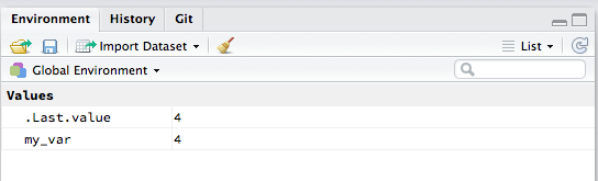
After defining a variable:
my_var <- 4we can see its value in the console:
print(my_var)
#> [1] 4

# or simply
my_var
#> [1] 4
Check the Environment pane. You should see new variables appearing there.
Practise defining some new variables.
vector <- c(1, 3, 4, 7, 11, 2)
sum_of_vector <- sum(vector)

mean_of_vector <- mean(vector)
mean_of_vector
#> [1] 4.666667

rounded_mean <- round(mean_of_vector, digits = 1)
rounded_mean
#> [1] 4.7
These variables exist in the Global Environment, but will no longer be available if we restart R. It makes sense to save everything we do in a text file.
2.3 Function calls
Let’s take a closer look at the syntax of R function calls.
The function shown below consists of a name function_name and two arguments, arg1 and arg2. The arguments may have default values. In this example, arg1 doesn’t have a default value, but arg2 has the default value val2. Arguments with no default value are required, whereas arguments with a default value are not. These simply take their default value if the a value is not explictly provided.
function_name(arg1, arg2 = val2)A function may have many arguments.
= vs. <- for function arguments.
# assignment:
# `<-` assigns a value to an object:
x <- c(23.192, 21.454, 24.677)
# or
x = c(23.192, 21.454, 24.677)

# arguments of functions:
# `=` for passing function arguments with values:
round(x, digits = 1)
#> [1] 23.2 21.5 24.7
The == operator is used in order to test for equivalance.
x1 <- 3
x2 <- 4
# is x1 equal to x2?
x1 == x2
#> [1] FALSE
Using tab completion for function arguments:
-
At the R prompt, enter
scale(and pressTAB. -
What are the arguments of the function
round()? Do any have default values? -
Look up the
rnorm()function in the Help Viewer. What arguments? Any default values? -
Do the same for the
seq()function. -
What do the following function calls do?
-
seq() -
seq(1, 10) -
seq(1, 10, 2) -
seq(1, 10, 2, 20) -
seq(1, 10, length.out = 20)
-
2.3.1 Nested function calls
Function calls can be nested. This means that the output of one function is passed as input to the next function.
For example: Let’s define a vector, campute its mean and then round to two decimal places:
# define a vector:
c(34.444, 45.853, 21.912, 29.261, 31.558)
#> [1] 34.444 45.853 21.912 29.261 31.558

# compute mean:
mean(c(34.444, 45.853, 21.912, 29.261, 31.558))
#> [1] 32.6056

# round:
round(mean(c(34.444, 45.853, 21.912, 29.261, 31.558)),
      digits = 2)
#> [1] 32.61
Function calls are always performed in the same order: from innermost to outermost, e.g. first mean() and then round().
2.4 Data types
Vectors are the fundamental data type in R - all other data types are composed of vectors. These can subdivided into:
numeric vectors: a further subdivision is into
integer(whole numbers) unddouble(floating point numbers).character vectors: these consist of characters strings and are surrounded by quotes, either single
'or double", e.g.'word'oder"word".logical vectors: these can take three values:
TRUE,FALSEorNA.
Vectors consist of elements of the same type, i.e., we cannot combine logical and character elements in a vector. Vectors have three properties:
- Type:
typeof(): what is it? - Length:
length(): how many elements? - Attribute:
attributes(): additional metadata
Vectors are created using the c() function or by using special function, such as seq() or rep().
2.4.1 Numeric vectors
Numeric vectors consist of integers or floating point numbers.
numbers <- c(1, 2.5, 4.5)
typeof(numbers)
#> [1] "double"
length(numbers)
#> [1] 3
We can subset vectors, i.e. select individual elements from a vector using []:
# the first element:
numbers[1]
#> [1] 1

# the sesond element:
numbers[2]
#> [1] 2.5

# the last element:
# numbers has length 3
length(numbers)
#> [1] 3

# we can use this for subsetting
numbers[length(numbers)]
#> [1] 4.5

# with - (minus) we can omit an element, e.g. the first
numbers[-1]
#> [1] 2.5 4.5

# we can use a sequence
numbers[1:2]
#> [1] 1.0 2.5

# we can omit the first and third elements
numbers[-c(1, 3)]
#> [1] 2.5
Matrices
A matrix is a special kind of vector in R. It has an additional dim (dimension) attribute:
# x is a vector
x <- 1:8

# we can define the dimensions of x
dim(x) <- c(2, 4)
x
#>      [,1] [,2] [,3] [,4]
#> [1,]    1    3    5    7
#> [2,]    2    4    6    8

# we can also create a matrix like this:
m <- matrix(x <- 1:8, nrow = 2, ncol = 4, byrow = FALSE)
m
#>      [,1] [,2] [,3] [,4]
#> [1,]    1    3    5    7
#> [2,]    2    4    6    8

# what are its dimensions?
dim(m)
#> [1] 2 4
We are using the argument byrow, which has the default value FALSE. If we set this to true (byrow = TRUE) we obtain:
m2 <- matrix(x <- 1:8, nrow = 2, ncol = 4, byrow = TRUE)
m2
#>      [,1] [,2] [,3] [,4]
#> [1,]    1    2    3    4
#> [2,]    5    6    7    8
Now, the rows are filled in first.
Matrices can be transposed, i.e. the rows become the columns and vice versa:
m_transposed <- t(m)
m_transposed
#>      [,1] [,2]
#> [1,]    1    2
#> [2,]    3    4
#> [3,]    5    6
#> [4,]    7    8
There are two further functions that are often used for creating matrices: cbind() and rbind().
cbind() combines columns of several objects:
x1 <- 1:3
# x1 is a vector
x1
#> [1] 1 2 3

x2 <- 10:12
# x2 is a vector
x2
#> [1] 10 11 12


m1 <- cbind(x1, x2)
# m1 is a matrix with dimensions [3, 2]
m1
#>      x1 x2
#> [1,]  1 10
#> [2,]  2 11
#> [3,]  3 12
You can try out something similar with rbind():
m2 <- rbind(x1, x2)
# m2 is a matrix with dimensions [2, 3]
m2
#>    [,1] [,2] [,3]
#> x1    1    2    3
#> x2   10   11   12
Matrices can be subset using []. Note that here we need to specify both rows and columns: [row, column], separated by a comma. If either row or column is omitted, R selects all rows or columns.
# row 1, column 1
m1[1, 1]
#> x1
#>  1

# row 1, column 2
m1[1, 2]
#> x2
#> 10

# rows 2-3, column 1
m1[2:3, 1]
#> [1] 2 3
# all rows, column 1
m1[, 1]
#> [1] 1 2 3
# row 2, all columns
m1[2, ]
#> x1 x2
#> 2 11Vectorization
Everything in R is vectorized, i.e. everything operates on vector:
x1 <- 1:10
x1 + 2
#>  [1]  3  4  5  6  7  8  9 10 11 12

x2 <- 11:20

x1 + x2
#>  [1] 12 14 16 18 20 22 24 26 28 30

x1 * x2
#>  [1]  11  24  39  56  75  96 119 144 171 200
The same applies to functions:
x1 <- 1:10

x1^2
#>  [1]   1   4   9  16  25  36  49  64  81 100

exp(x1)
#>  [1]     2.718282     7.389056    20.085537    54.598150   148.413159
#>  [6]   403.428793  1096.633158  2980.957987  8103.083928 22026.465795
Recycling
Something to be aware of is vector recycling: This means that a shorter vector is repeated, e.g. if we add two vectors.
# the shorter vector is recycled:
1:10 + 1:2
#>  [1]  2  4  4  6  6  8  8 10 10 12
This is what is happening here:
1  2  3  4  5  6  7  8  9 10
1  2  1  2  1  2  1  2  1  2
The vector 1:2 is repeated as often as necessary.
What happens if the length of the longer vector is not a mupliple of the length of the shorter vector?
1:10 + 1:3
#> Warning in 1:10 + 1:3: Länge des längeren Objektes
#>       ist kein Vielfaches der Länge des kürzeren Objektes
#>  [1]  2  4  6  5  7  9  8 10 12 11
R will give us a warning in this case.
1  2  3  4  5  6  7  8  9 10
1  2  3  1  2  3  1  2  3  1
Missing Values
Missing values are declared with NA.
numbers <- c(12, 13, 15, 11, NA, 10)
numbers
#> [1] 12 13 15 11 NA 10
We can use the function is.na() to test for missing values:
is.na(numbers)
#> [1] FALSE FALSE FALSE FALSE  TRUE FALSE
Missing values are not the same as Inf (infinity) and NaN (not a number). These occur for instance when you try to divide by zero: 1/0 or 0/0. A further data type is NULL; this is used when something should exist but remains undefined.
1/0
#> [1] Inf
0/0
#> [1] NaN
2.4.2 Character vectors
Character vectors (strings) are used to represent text:
text <- c("these are", "some strings")
text
#> [1] "these are"    "some strings"
typeof(text)
#> [1] "character"

# text has 2 elements:
length(text)
#> [1] 2
letters and LETTERS are so called built-in constants. They contain all letters in the English language.
?letters
letters[1:3]
#> [1] "a" "b" "c"
letters[10:15]
#> [1] "j" "k" "l" "m" "n" "o"
LETTERS[24:26]
#> [1] "X" "Y" "Z"
A useful function for creating character vectors is:
paste(LETTERS[1:3], letters[24:26], sep = "_")
#> [1] "A_x" "B_y" "C_z"

# special case with sep = ""
paste0(1:3, letters[5:7])
#> [1] "1e" "2f" "3g"

first_name <- "Ronald Aylmer"
last_name <- "Fisher"
paste("My name is:", first_name, last_name, sep = " ")
#> [1] "My name is: Ronald Aylmer Fisher"
2.4.3 Logical vectors
Logical vectors can take 3 values; TRUE, FALSE or NA.
log_var <- c(TRUE, FALSE, TRUE)
log_var
#> [1]  TRUE FALSE  TRUE
Logical vectors are used for indexing other vectors. For example, we might want to extract all elements of a vector that are greater than some value, e.g. all positive numbers.
set.seed(5434) # makes the example reproducible

# draw random numbers
x <- rnorm(24)
x
#>  [1]  1.06115528  0.87480990 -0.30032832  1.21965848  0.09860288
#>  [6]  1.89862128 -1.54699798  0.96349219 -0.64968432 -1.09672125
#> [11] -0.55326456 -0.29394388  0.58151046 -0.15135071  1.66997280
#> [16] -0.10726874  0.51633289 -0.64741465  0.10489022 -0.95484078
#> [21]  0.22940461 -0.54106301 -0.76310004  1.22446844

# we want all positive numbers:
x > 0
#>  [1]  TRUE  TRUE FALSE  TRUE  TRUE  TRUE FALSE  TRUE FALSE FALSE FALSE
#> [12] FALSE  TRUE FALSE  TRUE FALSE  TRUE FALSE  TRUE FALSE  TRUE FALSE
#> [23] FALSE  TRUE

# we can use this to index x:
x[x > 0]
#>  [1] 1.06115528 0.87480990 1.21965848 0.09860288 1.89862128 0.96349219
#>  [7] 0.58151046 1.66997280 0.51633289 0.10489022 0.22940461 1.22446844

# we can also save the index
index <- x > 0

# and use this:
x[index]
#>  [1] 1.06115528 0.87480990 1.21965848 0.09860288 1.89862128 0.96349219
#>  [7] 0.58151046 1.66997280 0.51633289 0.10489022 0.22940461 1.22446844
2.4.4 Factors
The numeric, logical, and character vectors we have met so far are atomic vectors, because they are the fundamental data types. For categorical data, used for grouping, we need a further object type. This is known as a factor. A factor is simply an vector of integers, with additional metadata (attributes). These consist of the object class factor and the factor levels.
# sex
sex <- c("male", "female", "male", "male", "female")
sex
#> [1] "male"   "female" "male"   "male"   "female"

typeof(sex)
#> [1] "character"

attributes(sex)
#> NULL
We can define a factor:
sex <- factor(sex, levels = c("female", "male"))
sex
#> [1] male   female male   male   female
#> Levels: female male

# sex hast type integer
typeof(sex)
#> [1] "integer"

# but `class` factor
class(sex)
#> [1] "factor"

# and attributes levels und class
attributes(sex)
#> $levels
#> [1] "female" "male"
#>
#> $class
#> [1] "factor"
If we don’t explicitly define the levels, R just uses alphabetical ordering.
We can obtain the integer values of a factor by using unclass().
sex
#> [1] male   female male   male   female
#> Levels: female male
unclass(sex)
#> [1] 2 1 2 2 1
#> attr(,"levels")
#> [1] "female" "male"
Factors are essential for regression models. For example, if we use dummy coding, the first factor level will automatically be chosen as the reference category. We can change the ordering using relevel() or factor().
Usingrelevel():
levels(sex)
#> [1] "female" "male"

# the result has to be reassigned to the variable
sex <- relevel(sex, ref = "male")
levels(sex)
#> [1] "male"   "female"
We can also use factor() but then we need to provide all levels:
sex <- factor(sex, levels = c("male", "female"))
sex
#> [1] male   female male   male   female
#> Levels: male female
2.4.5 Lists
The next data types are lists. Whereas atomic vectors must be composed of elements of the same type, lists can contain heterogeneous elements (including other lists).
We can define a list using the function list():
x <- list(1:3, "a", c(TRUE, FALSE, TRUE), c(2.3, 5.9))
x
#> [[1]]
#> [1] 1 2 3
#>
#> [[2]]
#> [1] "a"
#>
#> [[3]]
#> [1]  TRUE FALSE  TRUE
#>
#> [[4]]
#> [1] 2.3 5.9
This list contains a numeric vector, a character, a logical vector and another numeric vector.
# the type of a list is "list"
typeof(x)
#> [1] "list"
Lists can be indexed just like vectors:
x[1]
#> [[1]]
#> [1] 1 2 3
x[2]
#> [[1]]
#> [1] "a"
x[3]
#> [[1]]
#> [1]  TRUE FALSE  TRUE
x[4]
#> [[1]]
#> [1] 2.3 5.9
Lists can also be indexed using double square brackets, [[. This is explained very well in R for Data Science.
Lists are very important in R; most statistical functions actually create lists as outputs, and it is useful to know how to deal with these.
Lists can also have named elements:
x <- list(int = 1:3,
          string = "a",
          log = c(TRUE, FALSE, TRUE),
          double = c(2.3, 5.9))
x
#> $int
#> [1] 1 2 3
#>
#> $string
#> [1] "a"
#>
#> $log
#> [1]  TRUE FALSE  TRUE
#>
#> $double
#> [1] 2.3 5.9
x is a named list. This makes subsetting easier - there is a special operator, the $ operator, which can be used for selecting named elements of a list. This can be used together with tab completion. If you type x$ at the R prompt, R will show all named elements.
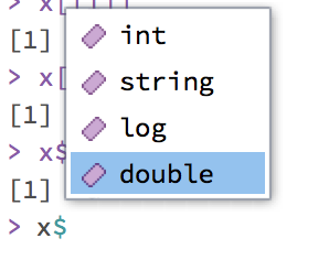
x$string
#> [1] "a"
x$double
#> [1] 2.3 5.9
2.4.6 Data frames
For statistics, data frames are the most important objects. They are used to represent data. A data frame is a two dimensional structure with rows and columns. Technically, a data frame is a list whose elements are equal lenght vectors. These vectors can be numeric, logical or character, or factors for grouping variables.
A data frame can be subset as a matrix, or as a list.
In RStudio, data frames are sometimes referred to as tibbles or tbl. tibbles are created using the function data_frame(), and are a more modern version of data frames.
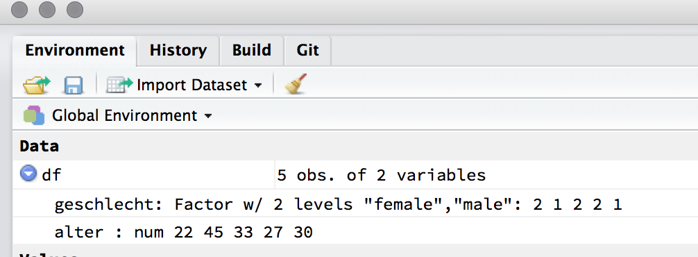
Let’s create a data frame. We will use the data_frame() function which is provided by the dplyr package.
library(dplyr)
df <- data_frame(sex = factor(c("male", "female",
                                       "male", "male",
                                       "female")),
                 age = c(22, 45, 33, 27, 30))
df
#> # A tibble: 5 x 2
#>   sex      age
#>   <fct>  <dbl>
#> 1 male    22.0
#> 2 female  45.0
#> 3 male    33.0
#> 4 male    27.0
#> 5 female  30.0
df is a data frame (or tibble) with two variables, sex and age. This data frame should appear in the Environment pane (under Data):
A data frame has the attributes names(), colnames() und rownames(); names() und colnames() refer to the same thing.
attributes(df)
#> $names
#> [1] "sex" "age"
#>
#> $row.names
#> [1] 1 2 3 4 5
#>
#> $class
#> [1] "tbl_df"     "tbl"        "data.frame"
The length of a data frame is the length of the list, i.e. the number of colummns. We can also use ncol(). To get the number of rows, we can use nrow().
ncol(df)
#> [1] 2
nrow(df)
#> [1] 5
Data frame subsetting
Data frames can be subset as a list, or as a matrix.
- as a list: columns (variables) can be selected using
$or[ - as a matrix: elements can be selected using
[
# choose variables
df$sex
#> [1] male   female male   male   female
#> Levels: female male

df$age
#> [1] 22 45 33 27 30

df["sex"]
#> # A tibble: 5 x 1
#>   sex
#>   <fct>
#> 1 male
#> 2 female
#> 3 male
#> 4 male
#> 5 female

df["age"]
#> # A tibble: 5 x 1
#>     age
#>   <dbl>
#> 1  22.0
#> 2  45.0
#> 3  33.0
#> 4  27.0
#> 5  30.0

# by position
df[1]
#> # A tibble: 5 x 1
#>   sex
#>   <fct>
#> 1 male
#> 2 female
#> 3 male
#> 4 male
#> 5 female

df[2]
#> # A tibble: 5 x 1
#>     age
#>   <dbl>
#> 1  22.0
#> 2  45.0
#> 3  33.0
#> 4  27.0
#> 5  30.0
We can also select rows and columns, just as we would do with a matrix: [row, column].
# row 1, column 1
df[1, 1]
#> # A tibble: 1 x 1
#>   sex
#>   <fct>
#> 1 male

# row 1, all columns
df[1, ]
#> # A tibble: 1 x 2
#>   sex     age
#>   <fct> <dbl>
#> 1 male   22.0

# all rows, column 1
df[, 1]
#> # A tibble: 5 x 1
#>   sex
#>   <fct>
#> 1 male
#> 2 female
#> 3 male
#> 4 male
#> 5 female

# all rows, all columns
df[ , ]
#> # A tibble: 5 x 2
#>   sex      age
#>   <fct>  <dbl>
#> 1 male    22.0
#> 2 female  45.0
#> 3 male    33.0
#> 4 male    27.0
#> 5 female  30.0

# first 3 rows, all columns
df[1:3, ]
#> # A tibble: 3 x 2
#>   sex      age
#>   <fct>  <dbl>
#> 1 male    22.0
#> 2 female  45.0
#> 3 male    33.0
We can also index individual columns (variables):
df$sex[1]
#> [1] male
#> Levels: female male
2.5 Exercises
Rounding numbers
x <- rnorm(10, mean = 1, sd = 0.5)
x
#>  [1]  0.66851021  1.60952322  0.62064523  0.62563620  1.31433575
#> [6] 1.10078969 0.48313164 -0.02969281 0.71076782 0.85972382- round the vector
xto 0 decimal places. - round the vector
xto 3 decimal places.
this_number <- 3.45263- Round the number
this_numberto the nearest whole number.
Compute mean
- In this data frame, compute the mean age:
df <- data_frame(sex = sample(c("male", "female"),
                                     size = 24,
                                     replace = TRUE),
                 age = runif(24, min = 19, max = 45))
df
#> # A tibble: 24 x 2
#>   sex      age
#>   <chr>  <dbl>
#> 1 male    22.1
#> 2 male    22.6
#> 3 male    24.4
#> 4 female  40.7
#> 5 male    22.0
#> 6 male    42.1
#> # ... with 18 more rows- Have a look at some summary statistics using the
summary()function.
Character vectors
Generate a new variable from the variables ID, initials and age using the paste() function. The new variable should look like this:
"1-RS-44" "2-MM-78" "3-PD-22" "4-PG-34" "5-DK-67" "1-RS-59"ID <- c(1, 2, 3, 4, 5)
intials <- c("RS", "MM", "PD", "PG", "DK")
age <- c(44, 78, 22, 34, 67, 59)Data frames
Change the order of the factor levels in the following data set. We want placebo to be the new reference category.
library(dplyr)
library(tidyr)

alc_aggr <- data_frame(no_alcohol = c(64, 58, 64),
                            placebo = c(74, 79, 72),
                            anti_placebo = c(71, 69, 67),
                            alcohol = c(69, 73, 74))
alc_aggr <- alc_aggr %>%
    gather(key = condition, value = aggression) %>%
    mutate(condition = factor(condition))
alc_aggr
#> # A tibble: 12 x 2
#> condition aggression
#> <fct> <dbl>
#> 1 no_alcohol 64.0
#> 2 no_alcohol 58.0
#> 3 no_alcohol 64.0
#> 4 placebo 74.0
#> 5 placebo 79.0
#> 6 placebo 72.0
#> # ... with 6 more rowslevels(alc_aggr$condition)
#> [1] "alcohol" "anti_placebo" "no_alcohol" "placebo"
alc_aggr$condition <- factor(alc_aggr$condition, levels = c("placebo",
"anti_placebo",
"no_alcohol",
"alcohol"))
levels(alc_aggr$condition)
#> [1] "placebo" "anti_placebo" "no_alcohol" "alcohol"
# alternative Lösung
alc_aggr$condition <- relevel(alc_aggr$condition, ref = "placebo")
levels(alc_aggr$condition)
#> [1] "placebo" "anti_placebo" "no_alcohol" "alcohol"Advanced exercise
- Select all even numbers from a numeric vector:
x <- seq(1, 20, by = 1)
x
#>  [1]  1  2  3  4  5  6  7  8  9 10 11 12 13 14 15 16 17 18 19 20
Hint: you will need to use the modulo operator
%%. Even numbers are divisible by 2, i.e. there is no remainder when diving by 2.
# we need the remainder when divided by 2 for each element of x:
x %% 2
#>  [1] 1 0 1 0 1 0 1 0 1 0 1 0 1 0 1 0 1 0 1 0
# we can create a logical vector to use as an index:
index <- x %% 2 == 0
index
#> [1] FALSE TRUE FALSE TRUE FALSE TRUE FALSE TRUE FALSE TRUE FALSE
#> [12] TRUE FALSE TRUE FALSE TRUE FALSE TRUE FALSE TRUE# we can use it to index x:
even_numbers <- x[index]
even_numbers
#> [1] 2 4 6 8 10 12 14 16 18 20- Do the same for the odd numbers.
Operators are used like this:
1 + 2; they are written between the operands (infix notation). Functions are used like this:abs(x); they are applied to arguments.