7 Descriptive Statistics
7.1 Summary statistics of all variables in a dataset
The function summary(data_frame) returns descriptive statistics for all variables in a dataset. For numeric variables, the minimum, maximum, quartiles, median, and mean values are returned, for factors the frequencies of the factor levels. In addition, the number of missing values for both variable types is displayed.
We first import our sample data set and assign the variables their scale level (i.e., defining factors as factors). Afterwards, we delete all single items from the data set since they are not needed now. This reduced data set, which we call westost_scales, is then saved as an .Rdata file in our data folder, so that we can load it next time without having to do all the import work again.
library(tidyverse)
library(haven)
westost <- read_sav("data/Beispieldatensatz.sav")
westost$ID <- as.factor(westost$ID)
westost$westost <- as_factor(westost$westost)
westost$geschlecht <- as_factor(westost$geschlecht)
westost$SES <- as_factor(westost$SES, ordered = TRUE)
westost$Deutsch <- as_factor(westost$Deutsch, ordered = TRUE)
westost$Mathe <- as_factor(westost$Mathe, ordered = TRUE)
westost$Fremdspr <- as_factor(westost$Fremdspr, ordered = TRUE)
westost$bildung_vater <- as_factor(westost$bildung_vater)
westost$bildung_mutter <- as_factor(westost$bildung_mutter)
westost$bildung_vater_b <- as_factor(westost$bildung_vater_b)
westost$bildung_mutter_b <- as_factor(westost$bildung_mutter_b)
save(westost, file = "data/westost.Rdata")

westost_scales <- westost %>% select (-c(T1_1:T7_12))

save(westost_scales, file = "data/westost_scales.Rdata")
load(file = "data/westost_scales.Rdata")
westost_scales
#> # A tibble: 286 x 33
#>   ID    westost geschlecht alter SES   Deutsch Mathe Fremdspr Schnitt
#>   <fct> <fct>   <fct>      <dbl> <ord> <ord>   <ord> <ord>      <dbl>
#> 1 2     West    männlich      14 unte… befrie… befr… ausreic…       4
#> 2 14    West    männlich      14 durc… befrie… befr… ausreic…       4
#> 3 15    West    männlich      14 durc… befrie… befr… befried…       4
#> 4 17    West    männlich      15 durc… befrie… befr… ausreic…       4
#> 5 18    West    männlich      14 durc… gut     gut   befried…       4
#> 6 19    West    männlich      15 über… befrie… befr… ausreic…       4
#> # … with 280 more rows, and 24 more variables: bildung_vater <fct>,
#> #   bildung_mutter <fct>, bildung_vater_b <fct>, bildung_mutter_b <fct>,
#> #   swk_akad <dbl>, swk_selbstreg <dbl>, swk_durch <dbl>,
#> #   swk_motselbst <dbl>, swk_sozharm <dbl>, swk_bez <dbl>,
#> #   unt_eltern <dbl>, unt_freunde <dbl>, sch_leistung <dbl>,
#> #   sch_bez <dbl>, sch_regeln <dbl>, ges_gerecht <dbl>, ges_nepot <dbl>,
#> #   leben_selbst <dbl>, leben_fam <dbl>, leben_schule <dbl>,
#> #   leben_freunde <dbl>, leben_gesamt <dbl>, stress_somat <dbl>,
#> #   stress_psych <dbl>
With summary() we now can get a descriptive overview of the dataset:
summary(westost_scales)
#>        ID      westost       geschlecht      alter
#>  1      :  1   West:143   männlich:152   Min.   :13.0
#>  2      :  1   Ost :143   weiblich:134   1st Qu.:14.0
#>  10     :  1                             Median :15.0
#>  11     :  1                             Mean   :14.7
#>  12     :  1                             3rd Qu.:15.0
#>  14     :  1                             Max.   :17.0
#>  (Other):280
#>                     SES              Deutsch             Mathe
#>  sehr niedrig         :  1   ungenügend  :  0   ungenügend  :  0
#>  unterdurchschnittlich:  4   mangelhaft  :  3   mangelhaft  : 11
#>  durchschnittlich     :186   ausreichend : 52   ausreichend : 55
#>  überdurchschnittlich : 69   befriedigend:112   befriedigend:111
#>  sehr hoch            : 24   gut         :100   gut         : 88
#>  NA's                 :  2   sehr gut    : 16   sehr gut    : 19
#>                              NA's        :  3   NA's        :  2
#>          Fremdspr      Schnitt
#>  ungenügend  :  0   Min.   :3.000
#>  mangelhaft  : 10   1st Qu.:4.000
#>  ausreichend : 39   Median :4.500
#>  befriedigend:103   Mean   :4.462
#>  gut         :102   3rd Qu.:5.000
#>  sehr gut    : 21   Max.   :6.000
#>  NA's        : 11   NA's   :6
#>                                        bildung_vater
#>  Hauptschulabschluss oder niedriger           :41
#>  Realschulabschluss (mittlere Reife)          :94
#>  Fachabitur, Abitur                           :41
#>  Fachhochschulabschluss, Universitätsabschluss:93
#>  NA's                                         :17
#>
#>
#>                                        bildung_mutter bildung_vater_b
#>  Hauptschulabschluss oder niedriger           :43     niedrig:135
#>  Realschulabschluss (mittlere Reife)          :95     hoch   :134
#>  Fachabitur, Abitur                           :50     NA's   : 17
#>  Fachhochschulabschluss, Universitätsabschluss:84
#>  NA's                                         :14
#>
#>
#>  bildung_mutter_b    swk_akad     swk_selbstreg     swk_durch
#>  niedrig:138      Min.   :2.429   Min.   :2.875   Min.   :1.000
#>  hoch   :134      1st Qu.:4.571   1st Qu.:4.750   1st Qu.:4.667
#>  NA's   : 14      Median :5.143   Median :5.250   Median :5.333
#>                   Mean   :5.098   Mean   :5.246   Mean   :5.285
#>                   3rd Qu.:5.571   3rd Qu.:5.875   3rd Qu.:6.000
#>                   Max.   :7.000   Max.   :7.000   Max.   :7.000
#>                                                   NA's   :1
#>  swk_motselbst    swk_sozharm       swk_bez        unt_eltern
#>  Min.   :3.200   Min.   :1.571   Min.   :3.333   Min.   :1.500
#>  1st Qu.:5.000   1st Qu.:4.857   1st Qu.:5.167   1st Qu.:5.333
#>  Median :5.400   Median :5.381   Median :5.667   Median :6.167
#>  Mean   :5.447   Mean   :5.280   Mean   :5.616   Mean   :5.872
#>  3rd Qu.:6.000   3rd Qu.:5.857   3rd Qu.:6.167   3rd Qu.:6.667
#>  Max.   :7.000   Max.   :7.000   Max.   :7.000   Max.   :7.000
#>                                                  NA's   :1
#>   unt_freunde     sch_leistung      sch_bez        sch_regeln
#>  Min.   :2.000   Min.   :1.667   Min.   :1.000   Min.   :1.750
#>  1st Qu.:5.500   1st Qu.:3.667   1st Qu.:3.163   1st Qu.:4.000
#>  Median :6.000   Median :4.333   Median :3.750   Median :4.925
#>  Mean   :5.928   Mean   :4.326   Mean   :3.820   Mean   :4.875
#>  3rd Qu.:6.667   3rd Qu.:5.000   3rd Qu.:4.500   3rd Qu.:5.750
#>  Max.   :7.000   Max.   :7.000   Max.   :7.000   Max.   :7.000
#>  NA's   :1       NA's   :2
#>   ges_gerecht      ges_nepot      leben_selbst     leben_fam
#>  Min.   :1.000   Min.   :1.000   Min.   :1.000   Min.   :1.000
#>  1st Qu.:3.500   1st Qu.:3.600   1st Qu.:5.000   1st Qu.:5.333
#>  Median :4.167   Median :4.400   Median :5.500   Median :6.000
#>  Mean   :4.160   Mean   :4.423   Mean   :5.433   Mean   :5.760
#>  3rd Qu.:5.000   3rd Qu.:5.200   3rd Qu.:6.000   3rd Qu.:6.667
#>  Max.   :6.667   Max.   :7.000   Max.   :7.000   Max.   :7.000
#>                  NA's   :3       NA's   :1       NA's   :2
#>   leben_schule   leben_freunde    leben_gesamt    stress_somat
#>  Min.   :1.333   Min.   :2.000   Min.   :2.909   Min.   :1.000
#>  1st Qu.:4.000   1st Qu.:5.500   1st Qu.:5.000   1st Qu.:2.167
#>  Median :4.667   Median :6.000   Median :5.455   Median :3.000
#>  Mean   :4.670   Mean   :5.898   Mean   :5.417   Mean   :3.020
#>  3rd Qu.:5.333   3rd Qu.:6.500   3rd Qu.:5.909   3rd Qu.:3.667
#>  Max.   :7.000   Max.   :7.000   Max.   :6.909   Max.   :7.000
#>  NA's   :1       NA's   :1       NA's   :1       NA's   :3
#>   stress_psych
#>  Min.   :1.000
#>  1st Qu.:2.167
#>  Median :2.917
#>  Mean   :2.989
#>  3rd Qu.:3.667
#>  Max.   :6.833
#>  NA's   :2
7.2 Descriptive statistics for nominal variables
7.2.1 Frequencies with table()
Using table() we can display the frequencies of the categories (factor levels) of a factor. This is particularly useful if we are interested in the combined frequencies of several factors as in a cross-tabulation.
table(westost_scales$bildung_vater)
#>
#>            Hauptschulabschluss oder niedriger
#>                                            41
#>           Realschulabschluss (mittlere Reife)
#>                                            94
#>                            Fachabitur, Abitur
#>                                            41
#> Fachhochschulabschluss, Universitätsabschluss
#>                                            93
table(westost_scales$bildung_vater_b, westost_scales$bildung_mutter_b)
#>
#>           niedrig hoch
#>   niedrig     102   32
#>   hoch         35   99
table(westost_scales$westost, westost_scales$bildung_mutter)
#>
#>        Hauptschulabschluss oder niedriger
#>   West                                 43
#>   Ost                                   0
#>
#>        Realschulabschluss (mittlere Reife) Fachabitur, Abitur
#>   West                                  52                 20
#>   Ost                                   43                 30
#>
#>        Fachhochschulabschluss, Universitätsabschluss
#>   West                                            26
#>   Ost                                             58
Let’s generate some frequency plots with ggplot2:
p <- westost_scales %>%
select(bildung_vater) %>%
drop_na() %>%
ggplot(aes(x = bildung_vater))
p + geom_bar(fill = "darkblue") +
xlab("Education of the Father") +
ylab("Frequency")
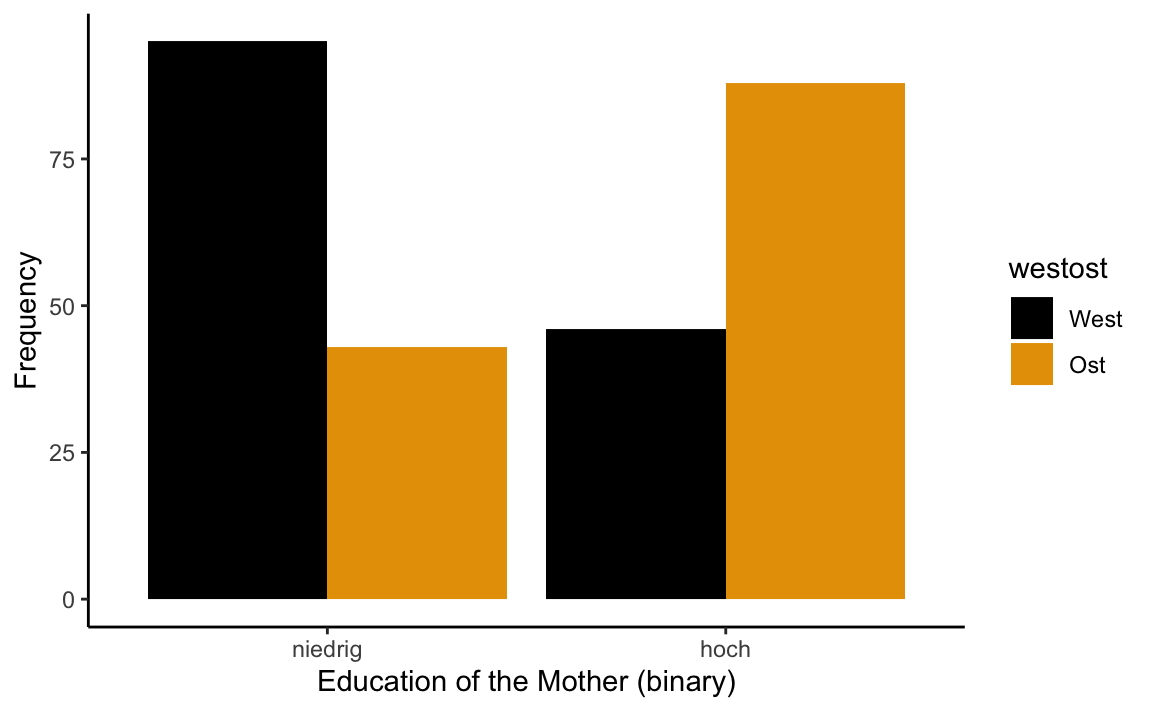
p1 <- westost_scales %>%
select(bildung_mutter_b, westost) %>%
drop_na() %>%
ggplot(aes(x = bildung_mutter_b, fill = westost))
p1 + geom_bar(position = "dodge") +
xlab("Education of the Mother (binary)") +
ylab("Frequency") +
theme_classic() +
scale_fill_manual(values = c("#000000", "#E69F00"))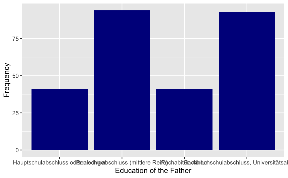
With prop.table() we can get proportions (relative frequencies):
table(westost_scales$bildung_vater_b, westost_scales$bildung_mutter_b) %>% prop.table() %>% round(2)
#>
#>           niedrig hoch
#>   niedrig    0.38 0.12
#>   hoch       0.13 0.37

# or in percentages

100*table(westost_scales$bildung_vater_b, westost_scales$bildung_mutter_b) %>% prop.table() %>% round(4)
#>
#>           niedrig  hoch
#>   niedrig   38.06 11.94
#>   hoch      13.06 36.94
In most cases we are not interested in the total proportions (which add up to 1 or 100% across the entire table), but in the row-conditional or column-conditional relative frequencies. The former are obtained using margin = 1 in the prop.table() function, the latter with margin = 2. Since there is no further argument, we can also directly specify the value of the argument, i.e. prop.table(1) for row-conditional proportions and prop.table(2) for column-conditional proportions.
table(westost_scales$geschlecht, westost_scales$westost)
#>
#>            West Ost
#>   männlich   83  69
#>   weiblich   60  74

# Relative frequencies (entire table)
table(westost_scales$geschlecht, westost_scales$westost) %>% prop.table() %>% round(2)
#>
#>            West  Ost
#>   männlich 0.29 0.24
#>   weiblich 0.21 0.26

# Row-conditional relative frequencies
table(westost_scales$geschlecht, westost_scales$westost) %>% prop.table(1) %>% round(2)
#>
#>            West  Ost
#>   männlich 0.55 0.45
#>   weiblich 0.45 0.55

# Column-conditional relative frequencies
table(westost_scales$geschlecht, westost_scales$westost) %>% prop.table(2) %>% round(2)
#>
#>            West  Ost
#>   männlich 0.58 0.48
#>   weiblich 0.42 0.52
7.2.2 Mode
There is no separate function for calculating the mode of a nominal variable. Either you read the mode (the category with the highest frequency) from the frequency table (or the frequency diagram), or you can help yourself with:
names(which.max(table(westost_scales$bildung_vater)))
#> [1] "Realschulabschluss (mittlere Reife)"
7.3 Descriptive statistics for ordinal and metric Variables
Most of the functions needed for describing the distributional characteristics of ordinal and metric variables we already know from the earlier chapter on the R language.
mean(x, na.rm = FALSE)    Arithmetic mean
sd(x)                     (Sample) Standard Deviation
var(x)                    (Sample) Variance

median(x)                 Median
quantile(x, probs, type)  Quantile of x.  probs: vector with probabilities
min(x)                    Minimum value of x
max(x)                    Maximum value of x
range(x)                  x_min and x_max
Examples
Let’s create a vector with 16 numbers between 1 and 9 and sort it:
x <- c(4, 7, 9, 2, 3, 6, 6, 4, 1, 2, 8, 5, 5, 7, 3, 2)
n <- length(x)
x <- sort(x)
x
#> [1] 1 2 2 2 3 3 4 4 5 5 6 6 7 7 8 9median(x)
#> [1] 4.5
quantile(x, c(.25, .75))
#> 25% 75%
#> 2.75 6.25The median = 4.5 corresponds to our expectations, as it is the mean of the 8th and 9th sorted values. The quartiles are \(Q_1=2.75\) and \(Q_3=6.25\)`. This is probably not what you’ve learned in your statistics course (at least not with us…). We have learned that if \(n\cdot p\) is not an integer, then the quantile is the \([(n\cdot p) + 1]\)th value of the distribution; on the other hand, if \(n\cdot p\) is an integer, the respective quantile is the mean of the \((n\cdot p)\)th and the \([(n\cdot p) + 1]\)th value. Since 16 can be devided by 4, both \(n\cdot 0.25\) and \(n\cdot 0.75\) are integers. Thus, the first quartile should be \(Q_1=\frac {x_{n \cdot 0.25}+x_{n \cdot 0.25+1}}{2} = \frac {x_4+x_5}{2}= \frac {2+3}{2}= 2.5\) and the third quartile should be \(Q_3=\frac {x_{n \cdot 0.75}+x_{n \cdot 0.75+1}}{2} = \frac {x_{12}+x_{13}}{2}= \frac {6 + 7}{2}= 6.5\). But that’s not what we obtained here…
The short and simple answer to this riddle is that quantile() has nine different methods (type = 1-9) to compute the quantiles of a distribution (help('quantile')). The default method is type = 7, but the method we prefer is type = 2. Therefore:
quantile(x, c(.25, .75), type = 2)
#> 25% 75%
#> 2.5 6.5
Which method is used by summary()?
summary(x)
#>    Min. 1st Qu.  Median    Mean 3rd Qu.    Max.
#>   1.000   2.750   4.500   4.625   6.250   9.000
Surprise! Summary also uses type = 7.
7.3.1 Descriptive summary of selected numerical variables
install.packages("RcmdrMisc")
Descriptive statistics for metric variables can be also obtained by the numSummary() function from the RcmdrMisc package.
The generic form of this function is: numSummary(df[, c("var1", "var2"], groups = df$factor, statistics = c("mean", "sd", "quantiles"), quantiles = c(0,.25,.5,.75,1)).
Additional statistics options are: se(mean) (standard error of the mean = \(\frac {sd}{\sqrt{n}}\)), cv (coefficient of variation = SD/mean), skewness, and kurtosis.
Example: Let us calculate descriptive statistics for the variables “Support by parents” (unt_eltern) and “Support by friends” (unt_friends) with mean value, standard deviation, standard error of the mean, skewness, kurtosis as well as the 10% and 90% quantiles. Using the groups argument we can do this separately for the levels of the factor (geschlecht).
library(RcmdrMisc)
numSummary(westost_scales[,c("unt_eltern", "unt_freunde")],
           groups = westost_scales$geschlecht,
           statistics = c("mean", "sd", "se(mean)", "skewness",
                          "kurtosis", "quantiles"),
           quantiles = c(.1,.9))
#>
#> Variable: unt_eltern
#>             mean        sd   se(mean)  skewness kurtosis      10%      90%
#> männlich 5.94415 0.8687628 0.07069892 -1.204500 1.088983 4.666667 6.833333
#> weiblich 5.79005 1.1232414 0.09703328 -1.332349 2.016779 4.333333 6.833333
#>            n NA
#> männlich 151  1
#> weiblich 134  0
#>
#> Variable: unt_freunde
#>              mean        sd   se(mean)   skewness  kurtosis      10%
#> männlich 5.584868 1.0055152 0.08155806 -0.8628965 0.8376967 4.333333
#> weiblich 6.319549 0.7416894 0.06431263 -2.2457703 8.4513611 5.500000
#>               90%   n NA
#> männlich 6.833333 152  0
#> weiblich 7.000000 133  1
p1 <- westost_scales %>%
select(unt_eltern, geschlecht) %>%
drop_na() %>%
ggplot(aes(x = unt_eltern, fill = geschlecht, y = ..density..))
p1 + geom_histogram(binwidth = 0.5,
position = "identity",
alpha = 0.5) +
scale_fill_manual(values = c("#000000", "#E69F00")) +
xlab("Support by Parents")
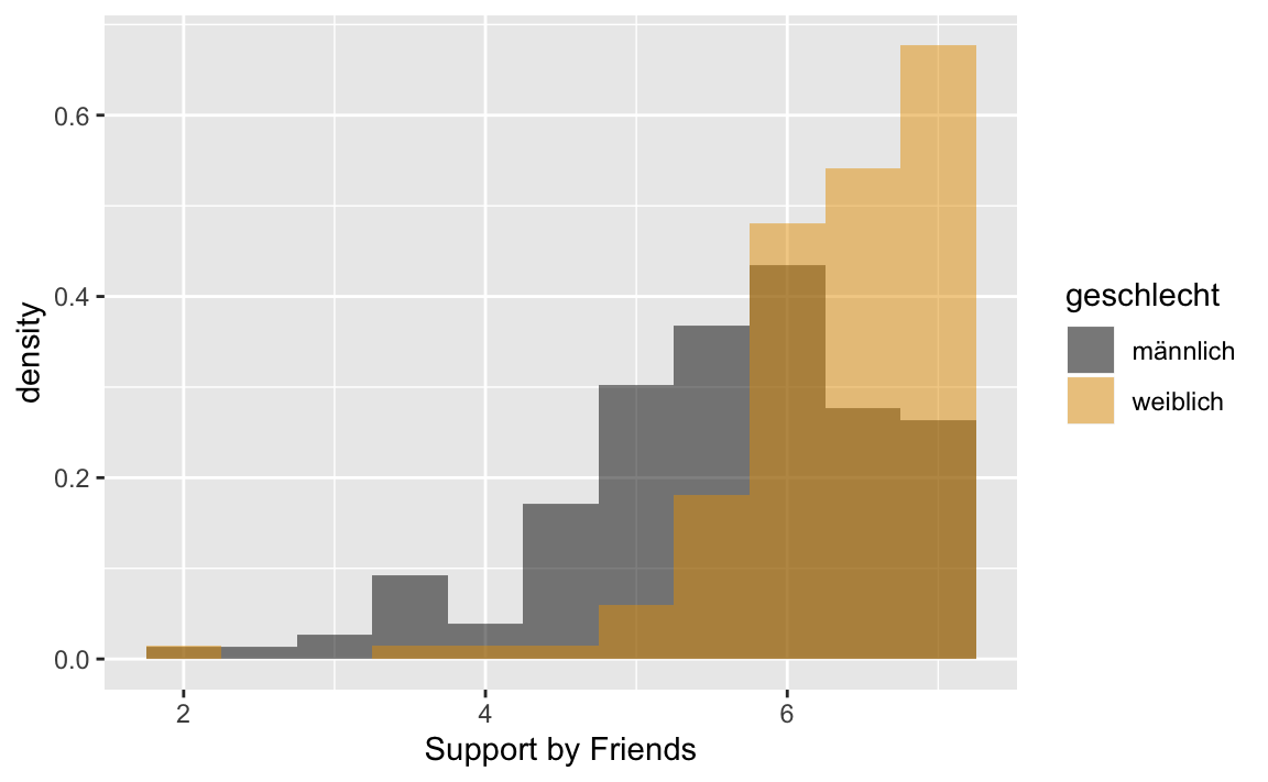
p2 <- westost_scales %>%
select(unt_freunde, geschlecht) %>%
drop_na() %>%
ggplot(aes(x = unt_freunde, fill = geschlecht, y = ..density..))
p2 + geom_histogram(binwidth = 0.5,
position = "identity",
alpha = 0.5) +
scale_fill_manual(values = c("#000000", "#E69F00"))+
xlab("Support by Friends")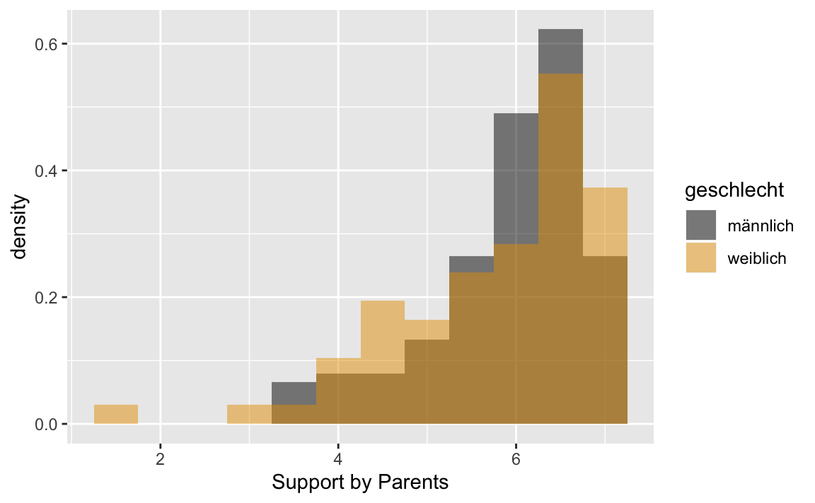
7.3.2 Table with statistics (tapply())
The tapply () function can be used to display selected descriptive statistics for the combined levels of several factors. Useful for the presentation of means in 2-factorial ANOVAS. The generic form is: tapply(df$var1, list(factor1 = df$factor1, factor2 = df$factor2), statistic, na.rm = TRUE).
statistic has to be replaced by the desired statistic (only one at a time), e.g. mean, median, sum, sd.
Let’s display the means of the variable “Support by Parents” for the combined factors geschlecht and westost:
tapply(westost_scales$unt_eltern,
       list(Geschlecht = westost_scales$geschlecht, Region = westost_scales$westost),
       mean, na.rm = TRUE) %>%
    round(2)
#>           Region
#> Geschlecht West  Ost
#>   männlich 5.79 6.13
#>   weiblich 5.74 5.83
We did the same already using dplyr:
westost_scales %>%
    group_by(geschlecht, westost) %>%
    summarise(mean = mean(unt_eltern, na.rm = TRUE))
#> # A tibble: 4 x 3
#> # Groups:   geschlecht [2]
#>   geschlecht westost  mean
#>   <fct>      <fct>   <dbl>
#> 1 männlich   West     5.79
#> 2 männlich   Ost      6.13
#> 3 weiblich   West     5.74
#> 4 weiblich   Ost      5.83

# Caution: If we use drop_na() to remove missing values, all cases with missings
# anywhere in the dataset will be removed. In this case, it is necessary to define
# a new dataset including only the relevant variables first!

westost_scales %>%
    group_by(geschlecht, westost) %>%
    drop_na() %>%
    summarise(mean = mean(unt_eltern))
#> # A tibble: 4 x 3
#> # Groups:   geschlecht [2]
#>   geschlecht westost  mean
#>   <fct>      <fct>   <dbl>
#> 1 männlich   West     5.78
#> 2 männlich   Ost      6.12
#> 3 weiblich   West     5.71
#> 4 weiblich   Ost      5.73
7.3.3 Descriptive statistics for metric variables using the psych package
install.packages("psych")
The psych package is often used for data analysis in psychology. It has a useful function for descriptive statistics for numerical variables: describe(). The generic form is: describe(x, na.rm = TRUE, interp = FALSE, skew = TRUE, ranges = TRUE, trim = .1, type = 3, check = TRUE).
x stands for the data frame or the variable to be analyzed (df$variable). The defaults are:
* interp = FALSE refers to the definition of the median (interp = TRUE uses our method of averaging adjacent values for an even n) * skew = TRUE displays skewness, kurtosis and the trimmed mean * ranges = TRUE displays the range * trim = .1 refers to the proportion of the distribution that is trimmed at the lower and upper ends for the trimmed mean (default trimming is 10% on both sides, thus the trimmed mean is computed from the middle 80% of the data) * type = 3 refers to the method of computing skewness and kurtosis (more here: ?psych::describe) * check = TRUE refers to checking for non-numeric variables in the dataset (for which describe has no use); if check = FALSE non-numeric variables exist, an error message is displayed.
library(psych)
describe(westost_scales)
#>                   vars   n   mean    sd median trimmed    mad   min    max
#> ID*                  1 286 143.50 82.71 143.50  143.50 106.01  1.00 286.00
#> westost*             2 286   1.50  0.50   1.50    1.50   0.74  1.00   2.00
#> geschlecht*          3 286   1.47  0.50   1.00    1.46   0.00  1.00   2.00
#> alter                4 286  14.70  0.76  15.00   14.65   1.48 13.00  17.00
#> SES*                 5 284   3.39  0.68   3.00    3.29   0.00  1.00   5.00
#> Deutsch*             6 283   4.26  0.86   4.00    4.27   1.48  2.00   6.00
#> Mathe*               7 284   4.17  0.95   4.00    4.18   1.48  2.00   6.00
#> Fremdspr*            8 275   4.31  0.93   4.00    4.33   1.48  2.00   6.00
#> Schnitt              9 280   4.46  0.69   4.50    4.51   0.74  3.00   6.00
#> bildung_vater*      10 269   2.69  1.10   2.00    2.74   1.48  1.00   4.00
#> bildung_mutter*     11 272   2.64  1.08   2.00    2.68   1.48  1.00   4.00
#> bildung_vater_b*    12 269   1.50  0.50   1.00    1.50   0.00  1.00   2.00
#> bildung_mutter_b*   13 272   1.49  0.50   1.00    1.49   0.00  1.00   2.00
#> swk_akad            14 286   5.10  0.77   5.14    5.11   0.85  2.43   7.00
#> swk_selbstreg       15 286   5.25  0.81   5.25    5.28   0.93  2.88   7.00
#> swk_durch           16 285   5.28  0.99   5.33    5.35   0.99  1.00   7.00
#> swk_motselbst       17 286   5.45  0.77   5.40    5.48   0.89  3.20   7.00
#> swk_sozharm         18 286   5.28  0.78   5.38    5.30   0.78  1.57   7.00
#> swk_bez             19 286   5.62  0.75   5.67    5.66   0.74  3.33   7.00
#> unt_eltern          20 285   5.87  1.00   6.17    6.01   0.74  1.50   7.00
#> unt_freunde         21 285   5.93  0.96   6.00    6.06   0.99  2.00   7.00
#> sch_leistung        22 284   4.33  1.20   4.33    4.33   0.99  1.67   7.00
#> sch_bez             23 286   3.82  1.12   3.75    3.82   1.00  1.00   7.00
#> sch_regeln          24 286   4.88  1.16   4.93    4.88   1.30  1.75   7.00
#> ges_gerecht         25 286   4.16  1.03   4.17    4.19   0.99  1.00   6.67
#> ges_nepot           26 283   4.42  1.09   4.40    4.43   1.19  1.00   7.00
#> leben_selbst        27 285   5.43  1.10   5.50    5.54   0.74  1.00   7.00
#> leben_fam           28 284   5.76  1.01   6.00    5.88   0.99  1.00   7.00
#> leben_schule        29 285   4.67  1.06   4.67    4.73   0.99  1.33   7.00
#> leben_freunde       30 285   5.90  0.81   6.00    5.95   0.74  2.00   7.00
#> leben_gesamt        31 285   5.42  0.69   5.45    5.46   0.67  2.91   6.91
#> stress_somat        32 283   3.02  1.19   3.00    2.93   0.99  1.00   7.00
#> stress_psych        33 284   2.99  1.20   2.92    2.91   1.11  1.00   6.83
#>                    range  skew kurtosis   se
#> ID*               285.00  0.00    -1.21 4.89
#> westost*            1.00  0.00    -2.01 0.03
#> geschlecht*         1.00  0.13    -1.99 0.03
#> alter               4.00  0.36    -0.36 0.04
#> SES*                4.00  0.91     0.73 0.04
#> Deutsch*            4.00 -0.09    -0.50 0.05
#> Mathe*              4.00 -0.15    -0.38 0.06
#> Fremdspr*           4.00 -0.35    -0.15 0.06
#> Schnitt             3.00 -0.41    -0.43 0.04
#> bildung_vater*      3.00 -0.06    -1.41 0.07
#> bildung_mutter*     3.00 -0.01    -1.34 0.07
#> bildung_vater_b*    1.00  0.01    -2.01 0.03
#> bildung_mutter_b*   1.00  0.03    -2.01 0.03
#> swk_akad            4.57 -0.16     0.02 0.05
#> swk_selbstreg       4.12 -0.35    -0.31 0.05
#> swk_durch           6.00 -0.80     1.45 0.06
#> swk_motselbst       3.80 -0.37    -0.32 0.05
#> swk_sozharm         5.43 -0.55     1.18 0.05
#> swk_bez             3.67 -0.48    -0.23 0.04
#> unt_eltern          5.50 -1.35     2.05 0.06
#> unt_freunde         5.00 -1.25     1.85 0.06
#> sch_leistung        5.33 -0.01    -0.37 0.07
#> sch_bez             6.00 -0.04    -0.05 0.07
#> sch_regeln          5.25 -0.10    -0.64 0.07
#> ges_gerecht         5.67 -0.26    -0.27 0.06
#> ges_nepot           6.00 -0.08    -0.10 0.06
#> leben_selbst        6.00 -1.28     2.41 0.07
#> leben_fam           6.00 -1.27     2.27 0.06
#> leben_schule        5.67 -0.48     0.11 0.06
#> leben_freunde       5.00 -1.16     3.10 0.05
#> leben_gesamt        4.00 -0.79     1.14 0.04
#> stress_somat        6.00  0.81     0.99 0.07
#> stress_psych        5.83  0.65     0.42 0.07
describe(westost_scales[, c("unt_eltern", "unt_freunde")])
#>             vars   n mean   sd median trimmed  mad min max range  skew
#> unt_eltern     1 285 5.87 1.00   6.17    6.01 0.74 1.5   7   5.5 -1.35
#> unt_freunde    2 285 5.93 0.96   6.00    6.06 0.99 2.0   7   5.0 -1.25
#>             kurtosis   se
#> unt_eltern      2.05 0.06
#> unt_freunde     1.85 0.06
describe(westost_scales[, c("unt_eltern", "unt_freunde")], trim = 0.2)
#>             vars   n mean   sd median trimmed  mad min max range  skew
#> unt_eltern     1 285 5.87 1.00   6.17    6.08 0.74 1.5   7   5.5 -1.35
#> unt_freunde    2 285 5.93 0.96   6.00    6.09 0.99 2.0   7   5.0 -1.25
#>             kurtosis   se
#> unt_eltern      2.05 0.06
#> unt_freunde     1.85 0.06
describe(westost_scales[, c("unt_eltern", "unt_freunde")], skew = FALSE,
         range = FALSE)
#>             vars   n mean   sd   se
#> unt_eltern     1 285 5.87 1.00 0.06
#> unt_freunde    2 285 5.93 0.96 0.06
mad stands for median average deviation (mean absolute deviation from the median, an alternative measure of dispersion). The variables recognized as factors are given a * in the table. Nevertheless, their (mostly useless) statistics are displayed in spite of the detection. We are mainly interested in the variables unt_eltern and unt_friends. With trim = 0.2 we request a trimmed mean where 20% of the values at the lower end of the distribution and 20% of the values at the upper end of the distribution are removed. Finally, with skew = FALSE, range = FALSE we request a descriptive statistic without skewness and kurtosis as well as without median, trimmed, mad, min, max, range.
7.4 Descriptive statistics with jmv
The package jmv is the R package for the fabulous new statistics program jamovi. Everything that can be done in jamovi can also be done directly in R. When jamovi is run in syntax mode it is even possible to copy-paste the generated R code directly into an R markdown document like this one.
For the example, let’s first get a dataset swk including all self-efficacy scales + the gender variable:
swk <- westost_scales %>%
    select(starts_with("swk"), "geschlecht")
names(swk)
#> [1] "swk_akad"      "swk_selbstreg" "swk_durch"     "swk_motselbst"
#> [5] "swk_sozharm"   "swk_bez"       "geschlecht"
Descriptive statistics can be obtained with descriptives().
library(jmv)
descriptives(
    data = swk,
    vars = c(
        "swk_akad",
        "swk_selbstreg",
        "swk_motselbst",
        "swk_durch",
        "swk_sozharm",
        "swk_bez"),
    splitBy = "geschlecht")
#>
#>  DESCRIPTIVES
#>
#>  Descriptives
#>  ──────────────────────────────────────────────────────────────────────────────────────────────────────────────
#>               geschlecht    swk_akad    swk_selbstreg    swk_motselbst    swk_durch    swk_sozharm    swk_bez
#>  ──────────────────────────────────────────────────────────────────────────────────────────────────────────────
#>    N          männlich           152              152              152          151            152        152
#>               weiblich           134              134              134          134            134        134
#>    Missing    männlich             0                0                0            1              0          0
#>               weiblich             0                0                0            0              0          0
#>    Mean       männlich          5.14             5.16             5.43         5.48           5.30       5.55
#>               weiblich          5.05             5.34             5.46         5.06           5.26       5.69
#>    Median     männlich          5.21             5.25             5.40         5.67           5.29       5.67
#>               weiblich          5.14             5.38             5.60         5.33           5.43       5.83
#>    Minimum    männlich          3.29             2.88             3.20         3.00           3.86       3.33
#>               weiblich          2.43             3.43             3.50         1.00           1.57       3.83
#>    Maximum    männlich          7.00             6.88             7.00         7.00           7.00       7.00
#>               weiblich          7.00             7.00             7.00         7.00           6.86       7.00
#>  ──────────────────────────────────────────────────────────────────────────────────────────────────────────────
With ?jmv::descriptives we get an overview of all the options:
descriptives(data, vars, splitBy = NULL, freq = FALSE, hist = FALSE,
  dens = FALSE, bar = FALSE, barCounts = FALSE, box = FALSE,
  violin = FALSE, dot = FALSE, dotType = "jitter", n = TRUE,
  missing = TRUE, mean = TRUE, median = TRUE, mode = FALSE,
  sum = FALSE, sd = FALSE, variance = FALSE, range = FALSE,
  min = TRUE, max = TRUE, se = FALSE, skew = FALSE, kurt = FALSE,
  quart = FALSE, pcEqGr = FALSE, pcNEqGr = 4)

Arguments

data        the data as a data frame
vars        a vector of strings naming the variables of interest in data
splitBy     a vector of strings naming the variables used to split vars
freq        TRUE or FALSE (default), provide frequency tables (nominal, ordinal
            variables only)
hist        TRUE or FALSE (default), provide histograms (continuous variables only)
dens        TRUE or FALSE (default), provide density plots (continuous variables only)
bar         TRUE or FALSE (default), provide bar plots (nominal, ordinal variables only)
barCounts   TRUE or FALSE (default), add counts to the bar plots
box         TRUE or FALSE (default), provide box plots (continuous variables only)
violin      TRUE or FALSE (default), provide violin plots (continuous variables only)
dot         TRUE or FALSE (default), provide dot plots (continuous variables only)

n           TRUE (default) or FALSE, provide the sample size
missing     TRUE (default) or FALSE, provide the number of missing values
mean        TRUE (default) or FALSE, provide the mean
median      TRUE (default) or FALSE, provide the median
mode        TRUE or FALSE (default), provide the mode
sum         TRUE or FALSE (default), provide the sum
sd          TRUE or FALSE (default), provide the standard deviation
variance    TRUE or FALSE (default), provide the variance
range       TRUE or FALSE (default), provide the range
min         TRUE (default) or FALSE, provide the minimum
max         TRUE (default) or FALSE, provide the maximum
se          TRUE or FALSE (default), provide the standard error
skew        TRUE or FALSE (default), provide the skewness
kurt        TRUE or FALSE (default), provide the kurtosis
quart       TRUE or FALSE (default), provide quartiles
pcEqGr      TRUE or FALSE (default), provide quantiles
pcNEqGr     an integer (default: 4) specifying the number of equal groups
Let’s try some of these:
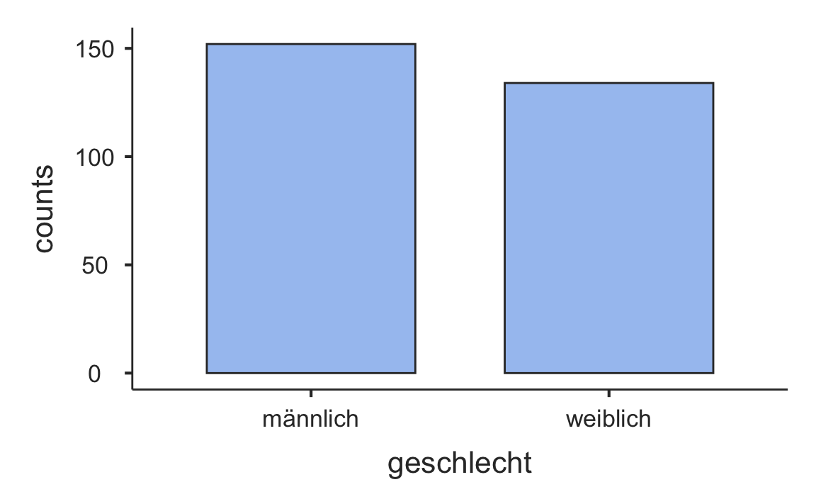
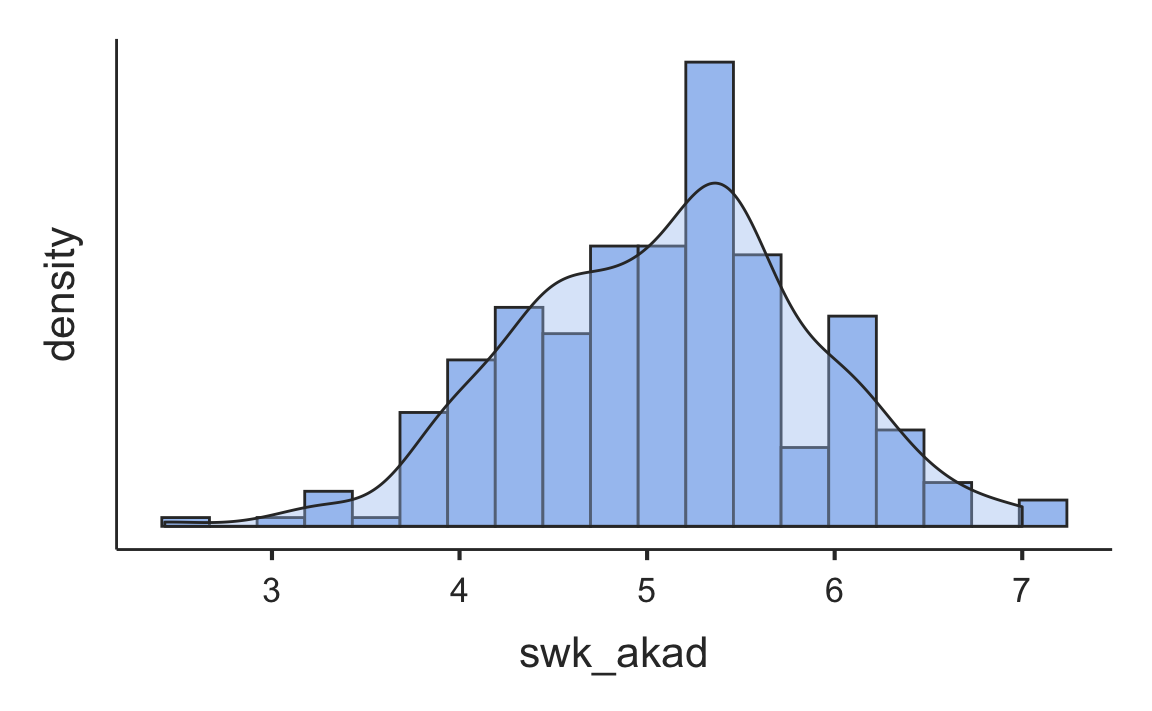
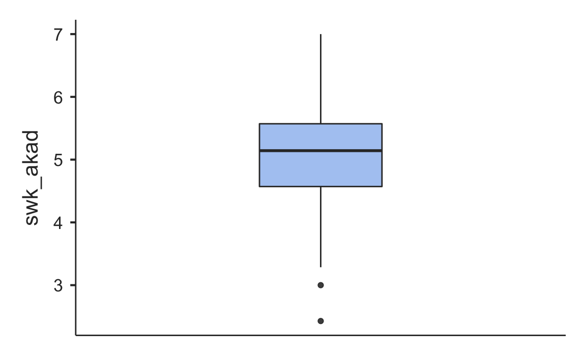
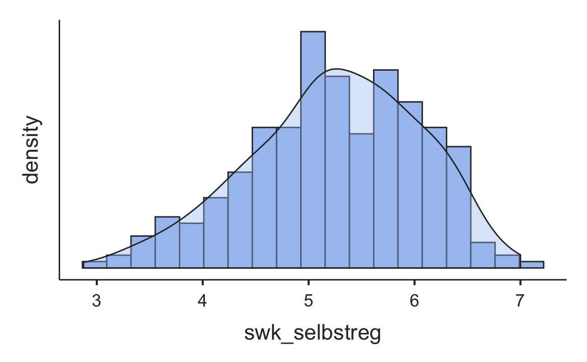
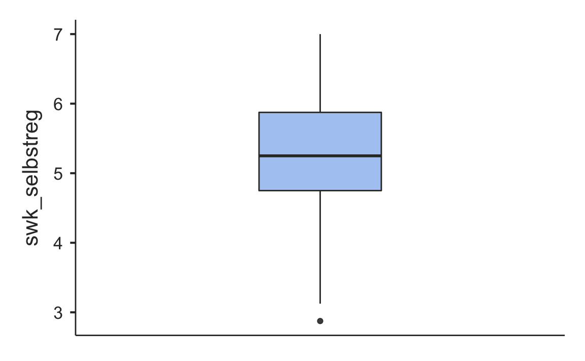
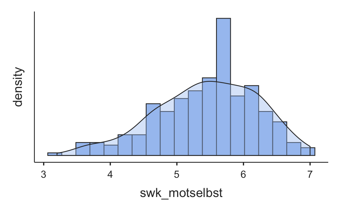
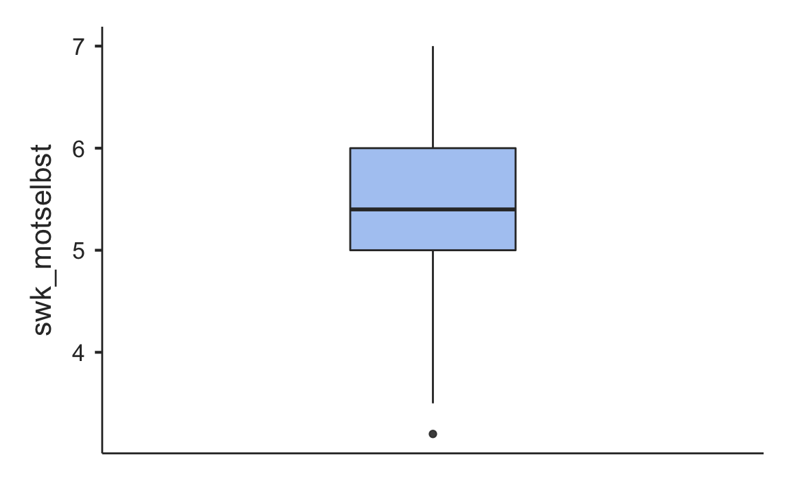
descriptives(
    data = swk,
    vars = c(
        "geschlecht",
        "swk_akad",
        "swk_selbstreg",
        "swk_motselbst"),
    freq = TRUE,
    hist = TRUE,
    dens = TRUE,
    bar = TRUE,
    barCounts = TRUE,
    box = TRUE,
    sd = TRUE,
    variance = TRUE,
    range = TRUE,
    se = TRUE,
    skew = TRUE,
    kurt = TRUE,
    quart = TRUE,
    pcEqGr = TRUE,
    pcNEqGr = 10
)
#>
#>  DESCRIPTIVES
#>
#>  Descriptives
#>  ───────────────────────────────────────────────────────────────────────────────────
#>                           geschlecht    swk_akad    swk_selbstreg    swk_motselbst
#>  ───────────────────────────────────────────────────────────────────────────────────
#>    N                             286         286              286              286
#>    Missing                         0           0                0                0
#>    Mean                                     5.10             5.25             5.45
#>    Std. error mean                        0.0455           0.0476           0.0454
#>    Median                                   5.14             5.25             5.40
#>    Standard deviation                      0.770            0.805            0.768
#>    Variance                                0.593            0.648            0.590
#>    Range                                    4.57             4.12             3.80
#>    Minimum                                  2.43             2.88             3.20
#>    Maximum                                  7.00             7.00             7.00
#>    Skewness                               -0.161           -0.359           -0.374
#>    Std. error skewness                     0.144            0.144            0.144
#>    Kurtosis                               0.0615           -0.279           -0.288
#>    Std. error kurtosis                     0.287            0.287            0.287
#>    25th percentile                          4.57             4.75             5.00
#>    50th percentile                          5.14             5.25             5.40
#>    75th percentile                          5.57             5.88             6.00
#>    10th percentile                          4.14             4.12             4.40
#>    20th percentile                          4.43             4.62             4.80
#>    30th percentile                          4.66             4.88             5.00
#>    40th percentile                          4.86             5.12             5.33
#>    50th percentile                          5.14             5.25             5.40
#>    60th percentile                          5.33             5.50             5.80
#>    70th percentile                          5.43             5.75             6.00
#>    80th percentile                          5.71             6.00             6.20
#>    90th percentile                          6.07             6.25             6.40
#>  ───────────────────────────────────────────────────────────────────────────────────
#>
#>
#>  FREQUENCIES
#>
#>  Frequencies of geschlecht
#>  ────────────────────────────────────────────────────
#>    Levels      Counts    % of Total    Cumulative %
#>  ────────────────────────────────────────────────────
#>    männlich       152          53.1            53.1
#>    weiblich       134          46.9           100.0
#>  ────────────────────────────────────────────────────
Some of the functionality of the jamovi program comes in modules. The functions in these modules are not included in the jmv package, but in additional packages like scatr.
A scatter plot can be obtained with scatr::scat().
library(scatr)
scat(
    data = swk,
    x = "swk_akad",
    y = "swk_selbstreg",
    group = "geschlecht",
    line = "linear")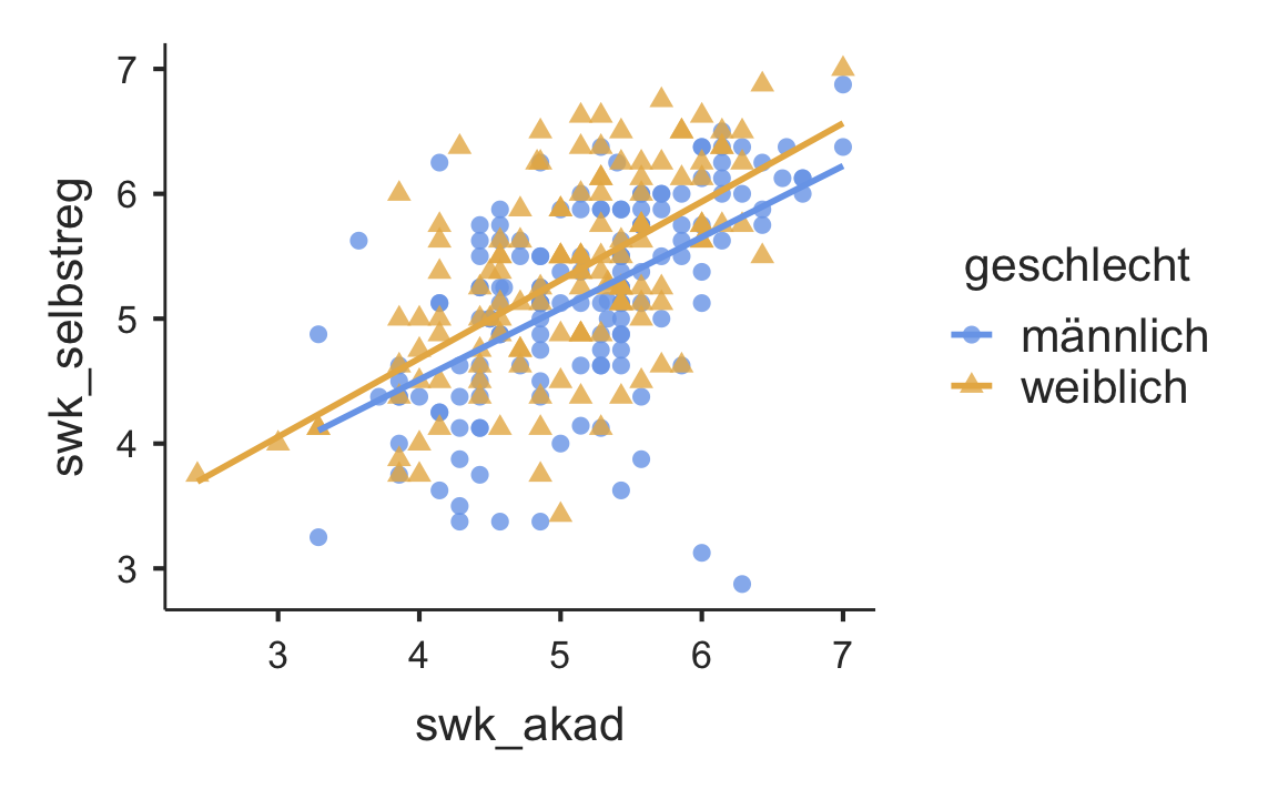
An overview of the available arguments is provided by ?scatr::scat:
scat(data, x, y, group = NULL, marg = "none", line = "none", se = FALSE)
Arguments

data    the data as a data frame
x       a string naming the variable from data that contains the x coordinates
        of the points in the plot, variable must be numeric
y       a string naming the variable from data that contains the y coordinates
        of the points in the plot, variable must be numeric
group   a string naming the variable from data that represents the grouping variable
marg    none (default), dens, or box, provide respectively no plots, density plots,
        or box plots on the axes
line    none (default), linear, or smooth, provide respectively no regression line,
        a linear regression line, or a smoothed regression line
se      TRUE or FALSE (default), show the standard error for the regression line
Let’s try some of these:
library(scatr)
scat(
    data = swk,
    x = "swk_akad",
    y = "swk_selbstreg",
    group = "geschlecht",
    marg = "dens",
    line = "smooth",
    se = TRUE)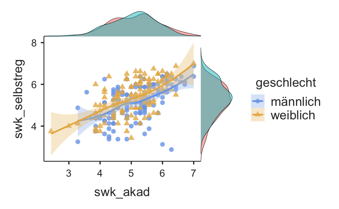
7.5 Correlations
7.5.1 Traditional ways of doing correlations in R
The generic form for calculating a (Pearson) correlation matrix using base R is as follows: cor(df[,c("var1", "var2", "var3")], methdod = c("pearson", "kendall", "spearman"), use = "complete.obs"). We can thus compute Pearson correlations (default) or - for ordinal data - Kendall’s tau or Spearman rank correlations.
swk_cor <- swk %>%
    select(-geschlecht) %>%
    cor(method = "pearson", use = "complete.obs") %>%
    round(3)
swk_cor
#>               swk_akad swk_selbstreg swk_durch swk_motselbst swk_sozharm
#> swk_akad         1.000         0.562     0.351         0.640       0.363
#> swk_selbstreg    0.562         1.000     0.318         0.724       0.342
#> swk_durch        0.351         0.318     1.000         0.415       0.592
#> swk_motselbst    0.640         0.724     0.415         1.000       0.407
#> swk_sozharm      0.363         0.342     0.592         0.407       1.000
#> swk_bez          0.392         0.466     0.327         0.415       0.493
#>               swk_bez
#> swk_akad        0.392
#> swk_selbstreg   0.466
#> swk_durch       0.327
#> swk_motselbst   0.415
#> swk_sozharm     0.493
#> swk_bez         1.000
If we want covariances instead of correlations we can use cov() with the same arguments as cor(): cov(df[,c(“var1”, “var2”, “var3”)], methdod = c(“pearson”, “kendall”, “spearman”), use = “complete.obs”).
A good way to display a scatterplot matrix for a number of variables is the function scatterplotMatrix from the car package. In addition to displaying all combinations of bivariate scatterplots it is possible to get different univariate plots in the diagonal: diagonal = c("density","boxplot","histogram","oned","qqplot","none"). Similar to scat() above, smooth = TRUE can be used to display a non-linear LOWESS line (LOcally WEighted Scatterplot Smoother) to assess the (non-)linearity of the correlation.
library(car)
scatterplotMatrix(~ swk_akad + swk_selbstreg + swk_sozharm +  swk_durch,
                  smooth = TRUE,
                  diagonal = "density",
                  data = swk)
#> Warning in applyDefaults(diagonal, defaults = list(method =
#> "adaptiveDensity"), : unnamed diag arguments, will be ignored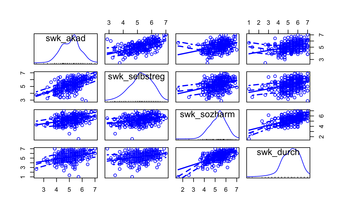
The function cor.test() can do a significance test for correlations, but only one at a time. The generic form is: cor. test (x, y, alternative = c ("two. sided", "less", "greater"), method = c ("pearson", "kendall", "spearman"), conf. level = 0.95). In addition to the non-directional alternative hypothesis (alternative = "two.sided"), we can also test directional alternative hypotheses: (alternative = "less") for a hypothesized negative correlation (“less than 0”) and (alternative = "greater") for a hypothesized positive correlation (“greater than 0”).
cor.test(swk$swk_akad, swk$swk_sozharm, alternative = "greater", method = "pearson")
#>
#>  Pearson's product-moment correlation
#>
#> data:  swk$swk_akad and swk$swk_sozharm
#> t = 6.5528, df = 284, p-value = 1.325e-10
#> alternative hypothesis: true correlation is greater than 0
#> 95 percent confidence interval:
#>  0.2746381 1.0000000
#> sample estimates:
#>       cor
#> 0.3624033
p <- swk %>%
select(swk_akad, swk_sozharm) %>%
drop_na() %>%
ggplot(mapping = aes(x = swk_akad,
y = swk_sozharm))
p + geom_jitter(size = 3, alpha = 0.6) +
stat_smooth(method = "lm", se = TRUE) +
theme_classic()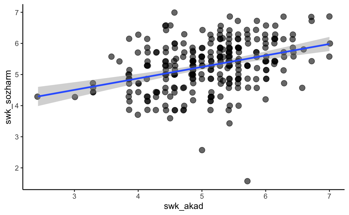
The function corr.test() from the psych package returns p-values for a correlation matrix. However, no directional alternative hypotheses are possible here. Matrices of correlations, sample sizes and p-values are displayed. With the p-value matrix, note that the unadjusted (two-sided) p-values are in the lower triangular matrix and the p-values adjusted according to Holm are in the upper triangular matrix. The Holm procedure corresponds to a sequential alpha correction that is less conservative than the Bonferroni procedure, but nevertheless controls the family-wise error. In the diagonals we also obtain p-values for the variances of the variables!
In the Holm procedure (Bonferroni-Holm method), the smallest p-value is multiplied by the number of tests (\(p(p-1)/2\); p = number of variables in the correlation matrix), the second smallest by the number of tests minus 1, etc. until the largest p-value that is no longer corrected (i.e., multiplied by \(p-p+1 = 1\)). However, the p-value is only multiplied by the corresponding number of tests if the resulting adjusted p-value is not smaller than the previously adjusted (smaller) p-value. If this is the case, the test is assigned the same p-value as its predecessor. This prevents that a smaller effect gets a smaller p-value after the adjustment than a larger effect, thereby preventing that a smaller effect may reach significance while the larger effect does not.
library(psych)
swk[1:25,] %>% select(starts_with("swk")) %>%
    corr.test()
#> Call:corr.test(x = .)
#> Correlation matrix
#>               swk_akad swk_selbstreg swk_durch swk_motselbst swk_sozharm
#> swk_akad          1.00          0.38      0.66          0.45        0.55
#> swk_selbstreg     0.38          1.00      0.47          0.70        0.37
#> swk_durch         0.66          0.47      1.00          0.41        0.72
#> swk_motselbst     0.45          0.70      0.41          1.00        0.49
#> swk_sozharm       0.55          0.37      0.72          0.49        1.00
#> swk_bez           0.31          0.56      0.34          0.66        0.66
#>               swk_bez
#> swk_akad         0.31
#> swk_selbstreg    0.56
#> swk_durch        0.34
#> swk_motselbst    0.66
#> swk_sozharm      0.66
#> swk_bez          1.00
#> Sample Size
#> [1] 25
#> Probability values (Entries above the diagonal are adjusted for multiple tests.)
#>               swk_akad swk_selbstreg swk_durch swk_motselbst swk_sozharm
#> swk_akad          0.00          0.23      0.00          0.14        0.04
#> swk_selbstreg     0.06          0.00      0.12          0.00        0.23
#> swk_durch         0.00          0.02      0.00          0.21        0.00
#> swk_motselbst     0.02          0.00      0.04          0.00        0.11
#> swk_sozharm       0.00          0.07      0.00          0.01        0.00
#> swk_bez           0.13          0.00      0.09          0.00        0.00
#>               swk_bez
#> swk_akad         0.23
#> swk_selbstreg    0.04
#> swk_durch        0.23
#> swk_motselbst    0.00
#> swk_sozharm      0.00
#> swk_bez          0.00
#>
#>  To see confidence intervals of the correlations, print with the short=FALSE option
7.5.2 Partial correlation
Partial correlations can be obtained partial.cor(df[, c("var1", "var2", "var3")], use = "complete.obs"). Important: Partialling for the corresponding bivariate correlation is done for all other variables in the data frame!
# Normal correlation matrix for comparison (zero-order correlations)
cor(westost_scales[,c("swk_akad", "swk_selbstreg", "Schnitt", "leben_schule")],
    use = "complete.obs")
#>                swk_akad swk_selbstreg   Schnitt leben_schule
#> swk_akad      1.0000000     0.5603931 0.4168517    0.3902735
#> swk_selbstreg 0.5603931     1.0000000 0.3824271    0.4896185
#> Schnitt       0.4168517     0.3824271 1.0000000    0.4754183
#> leben_schule  0.3902735     0.4896185 0.4754183    1.0000000

# Partial correlation matrix with three variables (first-order partial correlations)
partial.cor(westost_scales[,c("swk_akad", "swk_selbstreg", "Schnitt")],
            use = "complete.obs")
#>
#>  Partial correlations:
#>               swk_akad swk_selbstreg Schnitt
#> swk_akad       0.00000       0.47894 0.26472
#> swk_selbstreg  0.47894       0.00000 0.19889
#> Schnitt        0.26472       0.19889 0.00000
#>
#>  Number of observations: 280

# Partial correlation matrix with four variables (second-order partial correlations)
partial.cor(westost_scales[,c("swk_akad", "swk_selbstreg",
                              "Schnitt", "leben_schule")],
            use = "complete.obs")
#>
#>  Partial correlations:
#>               swk_akad swk_selbstreg Schnitt leben_schule
#> swk_akad       0.00000       0.43015 0.22486      0.07308
#> swk_selbstreg  0.43015       0.00000 0.07488      0.30949
#> Schnitt        0.22486       0.07488 0.00000      0.33116
#> leben_schule   0.07308       0.30949 0.33116      0.00000
#>
#>  Number of observations: 279
7.5.3 Correlation analysis with jmv
Almost all we have done above with the more traditional R functions we can also do in jmv using the corrMatrix() function:
library(jmv)
corrMatrix(
    data = swk,
    vars = c(
        "swk_akad",
        "swk_selbstreg",
        "swk_motselbst",
        "swk_durch",
        "swk_sozharm",
        "swk_bez"))
#>
#>  CORRELATION MATRIX
#>
#>  Correlation Matrix
#>  ─────────────────────────────────────────────────────────────────────────────────────────────────────────────────────
#>                                    swk_akad    swk_selbstreg    swk_motselbst    swk_durch    swk_sozharm    swk_bez
#>  ─────────────────────────────────────────────────────────────────────────────────────────────────────────────────────
#>    swk_akad         Pearson's r           —            0.562            0.641        0.351          0.362      0.391
#>                     p-value               —           < .001           < .001       < .001         < .001     < .001
#>
#>    swk_selbstreg    Pearson's r                            —            0.723        0.318          0.341      0.464
#>                     p-value                                —           < .001       < .001         < .001     < .001
#>
#>    swk_motselbst    Pearson's r                                             —        0.415          0.407      0.414
#>                     p-value                                                 —       < .001         < .001     < .001
#>
#>    swk_durch        Pearson's r                                                          —          0.592      0.327
#>                     p-value                                                              —         < .001     < .001
#>
#>    swk_sozharm      Pearson's r                                                                         —      0.493
#>                     p-value                                                                             —     < .001
#>
#>    swk_bez          Pearson's r                                                                                    —
#>                     p-value                                                                                        —
#>  ─────────────────────────────────────────────────────────────────────────────────────────────────────────────────────
An overview of the available arguments is provided by ?jmv::corrMatrix:
corrMatrix(data, vars, pearson = TRUE, spearman = FALSE, kendall = FALSE,
  sig = TRUE, flag = FALSE, ci = FALSE, ciWidth = 95, plots = FALSE,
  plotDens = FALSE, plotStats = FALSE, hypothesis = "corr")

Arguments

data        the data as a data frame
vars        a vector of strings naming the variables to correlate in data
pearson     TRUE (default) or FALSE, provide Pearson's R
spearman    TRUE or FALSE (default), provide Spearman's rho
kendall     TRUE or FALSE (default), provide Kendall's tau-b
sig         TRUE (default) or FALSE, provide significance levels
flag        TRUE or FALSE (default), flag significant correlations
ci          TRUE or FALSE (default), provide confidence intervals
ciWidth     a number between 50 and 99.9 (default: 95), the width of CI
plots       TRUE or FALSE (default), provide a correlation matrix plot
plotDens    TRUE or FALSE (default), provide densities in the correlation matrix plot
plotStats   TRUE or FALSE (default), provide statistics in the correlation matrix plot
hypothesis  one of 'corr' (default), 'pos', 'neg' specifying the alernative hypothesis;
            correlated, correlated positively, correlated negatively respectively.
Let’s try some options with only the three academic self-efficacy variables:
corrMatrix(
    data = swk,
    vars = c(
        "swk_akad",
        "swk_selbstreg",
        "swk_motselbst"),
    kendall = TRUE,
    sig = FALSE,
    flag = TRUE,
    ci = TRUE)
#>
#>  CORRELATION MATRIX
#>
#>  Correlation Matrix
#>  ──────────────────────────────────────────────────────────────────────────────────
#>                                        swk_akad    swk_selbstreg    swk_motselbst
#>  ──────────────────────────────────────────────────────────────────────────────────
#>    swk_akad         Pearson's r               —            0.562            0.641
#>                     95% CI Upper              —            0.636            0.704
#>                     95% CI Lower              —            0.477            0.567
#>                     Kendall's Tau B           —            0.425            0.471
#>
#>    swk_selbstreg    Pearson's r                                —            0.723
#>                     95% CI Upper                               —            0.774
#>                     95% CI Lower                               —            0.663
#>                     Kendall's Tau B                            —            0.569
#>
#>    swk_motselbst    Pearson's r                                                 —
#>                     95% CI Upper                                                —
#>                     95% CI Lower                                                —
#>                     Kendall's Tau B                                             —
#>  ──────────────────────────────────────────────────────────────────────────────────
#>    Note. * p < .05, ** p < .01, *** p < .001
7.6 Reliability analysis
7.6.1 Reliability analysis using the psych package
For the reliability analysis we will need the data set containing all individual items (westost). Then we create two reduced data sets: One for the scale “Self-Efficacy: Academic Achievement” (swkakad) including items T1_1, T1_7, T1_14, T1_16, T1_26, T1_27, and T1_31. And another for the scale “Self-Efficacy: Social Harmony” (swksozharm) including items T1_2, T1_8, T1_15, T1_23, T1_29, T1_32, and T1_35.
library(psych)
load(file = "data/westost.Rdata")
names(westost)
#>   [1] "ID"               "westost"          "geschlecht"
#>   [4] "alter"            "T1_1"             "T1_2"
#>   [7] "T1_3"             "T1_4"             "T1_5"
#>  [10] "T1_6"             "T1_7"             "T1_8"
#>  [13] "T1_9"             "T1_10"            "T1_11"
#>  [16] "T1_12"            "T1_13"            "T1_14"
#>  [19] "T1_15"            "T1_16"            "T1_17"
#>  [22] "T1_18"            "T1_19"            "T1_20"
#>  [25] "T1_21"            "T1_22"            "T1_23"
#>  [28] "T1_24"            "T1_25"            "T1_26"
#>  [31] "T1_27"            "T1_28"            "T1_29"
#>  [34] "T1_30"            "T1_31"            "T1_32"
#>  [37] "T1_33"            "T1_34"            "T1_35"
#>  [40] "T1_36"            "T2_1"             "T2_2"
#>  [43] "T2_3"             "T2_4"             "T2_5"
#>  [46] "T2_6"             "T3_1"             "T3_2"
#>  [49] "T3_3"             "T3_4"             "T3_5"
#>  [52] "T3_6"             "T4_1"             "T4_2"
#>  [55] "T4_3"             "T4_4"             "T4_5"
#>  [58] "T4_6"             "T4_7"             "T4_8"
#>  [61] "T4_9"             "T4_10"            "T4_11"
#>  [64] "T5_1"             "T5_2"             "T5_3"
#>  [67] "T5_4"             "T5_5"             "T5_6"
#>  [70] "T5_7"             "T5_8"             "T5_9"
#>  [73] "T5_10"            "T5_11"            "T6_1"
#>  [76] "T6_2"             "T6_3"             "T6_4"
#>  [79] "T6_5"             "T6_6"             "T6_7"
#>  [82] "T6_8"             "T6_9"             "T6_10"
#>  [85] "T6_11"            "T7_1"             "T7_2"
#>  [88] "T7_3"             "T7_4"             "T7_5"
#>  [91] "T7_6"             "T7_7"             "T7_8"
#>  [94] "T7_9"             "T7_10"            "T7_11"
#>  [97] "T7_12"            "SES"              "Deutsch"
#> [100] "Mathe"            "Fremdspr"         "Schnitt"
#> [103] "bildung_vater"    "bildung_mutter"   "bildung_vater_b"
#> [106] "bildung_mutter_b" "swk_akad"         "swk_selbstreg"
#> [109] "swk_durch"        "swk_motselbst"    "swk_sozharm"
#> [112] "swk_bez"          "unt_eltern"       "unt_freunde"
#> [115] "sch_leistung"     "sch_bez"          "sch_regeln"
#> [118] "ges_gerecht"      "ges_nepot"        "leben_selbst"
#> [121] "leben_fam"        "leben_schule"     "leben_freunde"
#> [124] "leben_gesamt"     "stress_somat"     "stress_psych"

swkakad <- westost %>%
    select(one_of(c("T1_1", "T1_7", "T1_14", "T1_16",
                    "T1_26", "T1_27", "T1_31")))
swkakad
#> # A tibble: 286 x 7
#>    T1_1  T1_7 T1_14 T1_16 T1_26 T1_27 T1_31
#>   <dbl> <dbl> <dbl> <dbl> <dbl> <dbl> <dbl>
#> 1     4     5     5     7     5     4     5
#> 2     3     5     5     7     4     5     5
#> 3     4     1     2     6     6     5     4
#> 4     6     5     6     7     7     6     6
#> 5     5     5     4     6     6     4     6
#> 6     6     5     6     7     7     3     4
#> # … with 280 more rows


swksozharm <- westost %>%
    select(one_of(c("T1_2", "T1_8", "T1_15", "T1_23",
                    "T1_29", "T1_32", "T1_35")))
swksozharm
#> # A tibble: 286 x 7
#>    T1_2  T1_8 T1_15 T1_23 T1_29 T1_32 T1_35
#>   <dbl> <dbl> <dbl> <dbl> <dbl> <dbl> <dbl>
#> 1     6     6     5     5     5     6     6
#> 2     5     6     4     3     4     6     5
#> 3     3     6     4     3     3     5     7
#> 4     6     6     6     6     6     6     6
#> 5     3     4     3     4     4     6     5
#> 6     6     6     6     5     7     7     7
#> # … with 280 more rows
Cronbach’s alpha
The internal consistency (Cronbach’s Alpha) can be computed using the function alpha():
alpha(swkakad)
#>
#> Reliability analysis
#> Call: alpha(x = swkakad)
#>
#>   raw_alpha std.alpha G6(smc) average_r S/N   ase mean   sd median_r
#>       0.63      0.63    0.65      0.19 1.7 0.033  5.1 0.77     0.18
#>
#>  lower alpha upper     95% confidence boundaries
#> 0.56 0.63 0.7
#>
#>  Reliability if an item is dropped:
#>       raw_alpha std.alpha G6(smc) average_r S/N alpha se var.r med.r
#> T1_1       0.59      0.59    0.60      0.19 1.4    0.037 0.022 0.168
#> T1_7       0.58      0.58    0.57      0.19 1.4    0.039 0.013 0.192
#> T1_14      0.57      0.56    0.57      0.18 1.3    0.039 0.022 0.097
#> T1_16      0.64      0.64    0.65      0.23 1.8    0.032 0.020 0.192
#> T1_26      0.61      0.61    0.63      0.21 1.6    0.035 0.024 0.180
#> T1_27      0.58      0.58    0.59      0.19 1.4    0.039 0.021 0.168
#> T1_31      0.56      0.57    0.56      0.18 1.3    0.040 0.015 0.180
#>
#>  Item statistics
#>         n raw.r std.r r.cor r.drop mean  sd
#> T1_1  286  0.53  0.56  0.45   0.34  5.0 1.2
#> T1_7  284  0.61  0.58  0.52   0.39  5.0 1.5
#> T1_14 283  0.61  0.62  0.54   0.41  4.9 1.4
#> T1_16 285  0.43  0.43  0.24   0.18  5.8 1.4
#> T1_26 285  0.47  0.50  0.34   0.27  5.3 1.2
#> T1_27 281  0.61  0.58  0.48   0.38  4.9 1.5
#> T1_31 283  0.63  0.61  0.56   0.43  4.7 1.4
#>
#> Non missing response frequency for each item
#>          1    2    3    4    5    6    7 miss
#> T1_1  0.01 0.01 0.07 0.20 0.33 0.30 0.08 0.00
#> T1_7  0.02 0.04 0.12 0.13 0.29 0.24 0.16 0.01
#> T1_14 0.03 0.05 0.07 0.19 0.26 0.32 0.10 0.01
#> T1_16 0.02 0.02 0.03 0.09 0.15 0.32 0.36 0.00
#> T1_26 0.01 0.01 0.05 0.14 0.31 0.33 0.15 0.00
#> T1_27 0.04 0.03 0.09 0.21 0.23 0.26 0.15 0.02
#> T1_31 0.03 0.03 0.13 0.22 0.26 0.23 0.10 0.01
Optionally, a “key vector” can be defined. This is particularly useful if you have some items that have been formulated in the opposite direction and therefore should actually be recoded before doing the reliability analysis. The “key vector” indicates which items have to be recoded (here: none!)
alpha(swkakad, keys = c(1, 1, 1, 1, 1, 1, 1))
#>
#> Reliability analysis
#> Call: alpha(x = swkakad, keys = c(1, 1, 1, 1, 1, 1, 1))
#>
#>   raw_alpha std.alpha G6(smc) average_r S/N   ase mean   sd median_r
#>       0.63      0.63    0.65      0.19 1.7 0.033  5.1 0.77     0.18
#>
#>  lower alpha upper     95% confidence boundaries
#> 0.56 0.63 0.7
#>
#>  Reliability if an item is dropped:
#>       raw_alpha std.alpha G6(smc) average_r S/N alpha se var.r med.r
#> T1_1       0.59      0.59    0.60      0.19 1.4    0.037 0.022 0.168
#> T1_7       0.58      0.58    0.57      0.19 1.4    0.039 0.013 0.192
#> T1_14      0.57      0.56    0.57      0.18 1.3    0.039 0.022 0.097
#> T1_16      0.64      0.64    0.65      0.23 1.8    0.032 0.020 0.192
#> T1_26      0.61      0.61    0.63      0.21 1.6    0.035 0.024 0.180
#> T1_27      0.58      0.58    0.59      0.19 1.4    0.039 0.021 0.168
#> T1_31      0.56      0.57    0.56      0.18 1.3    0.040 0.015 0.180
#>
#>  Item statistics
#>         n raw.r std.r r.cor r.drop mean  sd
#> T1_1  286  0.53  0.56  0.45   0.34  5.0 1.2
#> T1_7  284  0.61  0.58  0.52   0.39  5.0 1.5
#> T1_14 283  0.61  0.62  0.54   0.41  4.9 1.4
#> T1_16 285  0.43  0.43  0.24   0.18  5.8 1.4
#> T1_26 285  0.47  0.50  0.34   0.27  5.3 1.2
#> T1_27 281  0.61  0.58  0.48   0.38  4.9 1.5
#> T1_31 283  0.63  0.61  0.56   0.43  4.7 1.4
#>
#> Non missing response frequency for each item
#>          1    2    3    4    5    6    7 miss
#> T1_1  0.01 0.01 0.07 0.20 0.33 0.30 0.08 0.00
#> T1_7  0.02 0.04 0.12 0.13 0.29 0.24 0.16 0.01
#> T1_14 0.03 0.05 0.07 0.19 0.26 0.32 0.10 0.01
#> T1_16 0.02 0.02 0.03 0.09 0.15 0.32 0.36 0.00
#> T1_26 0.01 0.01 0.05 0.14 0.31 0.33 0.15 0.00
#> T1_27 0.04 0.03 0.09 0.21 0.23 0.26 0.15 0.02
#> T1_31 0.03 0.03 0.13 0.22 0.26 0.23 0.10 0.01
The following command is (erroneously) specified with recoding keys on variables 2 and 5:
alpha(swkakad, keys = c(1, -1, 1, 1, -1, 1, 1))
#>
#> Reliability analysis
#> Call: alpha(x = swkakad, keys = c(1, -1, 1, 1, -1, 1, 1))
#>
#>   raw_alpha std.alpha G6(smc) average_r S/N   ase mean   sd median_r
#>       0.63      0.63    0.65      0.19 1.7 0.033  5.1 0.77     0.18
#>
#>  lower alpha upper     95% confidence boundaries
#> 0.56 0.63 0.7
#>
#>  Reliability if an item is dropped:
#>       raw_alpha std.alpha G6(smc) average_r S/N alpha se var.r med.r
#> T1_1       0.59      0.59    0.60      0.19 1.4    0.037 0.022 0.168
#> T1_7       0.58      0.58    0.57      0.19 1.4    0.039 0.013 0.192
#> T1_14      0.57      0.56    0.57      0.18 1.3    0.039 0.022 0.097
#> T1_16      0.64      0.64    0.65      0.23 1.8    0.032 0.020 0.192
#> T1_26      0.61      0.61    0.63      0.21 1.6    0.035 0.024 0.180
#> T1_27      0.58      0.58    0.59      0.19 1.4    0.039 0.021 0.168
#> T1_31      0.56      0.57    0.56      0.18 1.3    0.040 0.015 0.180
#>
#>  Item statistics
#>         n raw.r std.r r.cor r.drop mean  sd
#> T1_1  286  0.53  0.56  0.45   0.34  5.0 1.2
#> T1_7  284  0.61  0.58  0.52   0.39  5.0 1.5
#> T1_14 283  0.61  0.62  0.54   0.41  4.9 1.4
#> T1_16 285  0.43  0.43  0.24   0.18  5.8 1.4
#> T1_26 285  0.47  0.50  0.34   0.27  5.3 1.2
#> T1_27 281  0.61  0.58  0.48   0.38  4.9 1.5
#> T1_31 283  0.63  0.61  0.56   0.43  4.7 1.4
#>
#> Non missing response frequency for each item
#>          1    2    3    4    5    6    7 miss
#> T1_1  0.01 0.01 0.07 0.20 0.33 0.30 0.08 0.00
#> T1_7  0.02 0.04 0.12 0.13 0.29 0.24 0.16 0.01
#> T1_14 0.03 0.05 0.07 0.19 0.26 0.32 0.10 0.01
#> T1_16 0.02 0.02 0.03 0.09 0.15 0.32 0.36 0.00
#> T1_26 0.01 0.01 0.05 0.14 0.31 0.33 0.15 0.00
#> T1_27 0.04 0.03 0.09 0.21 0.23 0.26 0.15 0.02
#> T1_31 0.03 0.03 0.13 0.22 0.26 0.23 0.10 0.01
Explanation of the output:
raw_alpha   # (Normal) Alpha based on covariances
std.alpha   # Standardized Alpha based on correlations
G6(smc)     # Guttman's Lambda 6 (alternative measure of reliability)
average_r   # Average inter-item-correlation
mean        # Scale mean (across all items)
sd          # Scale standard deviation
alpha.drop  # Statistics in case the respective item is deleted from the scale
item.stats # Item-total correlations (for raw and corrected scores) alpha(swksozharm)
#>
#> Reliability analysis
#> Call: alpha(x = swksozharm)
#>
#> raw_alpha std.alpha G6(smc) average_r S/N ase mean sd median_r
#> 0.8 0.82 0.81 0.39 4.5 0.018 5.3 0.78 0.36
#>
#> lower alpha upper 95% confidence boundaries
#> 0.77 0.8 0.84
#>
#> Reliability if an item is dropped:
#> raw_alpha std.alpha G6(smc) average_r S/N alpha se var.r med.r
#> T1_2 0.76 0.78 0.76 0.37 3.5 0.022 0.011 0.32
#> T1_8 0.76 0.78 0.76 0.37 3.5 0.022 0.012 0.32
#> T1_15 0.79 0.80 0.79 0.41 4.1 0.020 0.017 0.37
#> T1_23 0.82 0.82 0.81 0.44 4.6 0.016 0.011 0.39
#> T1_29 0.78 0.80 0.79 0.40 4.1 0.020 0.018 0.35
#> T1_32 0.77 0.78 0.77 0.37 3.5 0.022 0.013 0.35
#> T1_35 0.77 0.78 0.76 0.37 3.6 0.022 0.011 0.36
#>
#> Item statistics
#> n raw.r std.r r.cor r.drop mean sd
#> T1_2 285 0.75 0.75 0.71 0.61 5.2 1.27
#> T1_8 281 0.75 0.76 0.71 0.63 5.5 1.10
#> T1_15 284 0.64 0.64 0.54 0.49 4.7 1.10
#> T1_23 278 0.60 0.55 0.42 0.37 4.5 1.47
#> T1_29 286 0.65 0.65 0.56 0.51 5.1 1.10
#> T1_32 281 0.73 0.75 0.70 0.62 5.8 0.99
#> T1_35 281 0.72 0.75 0.71 0.62 6.1 0.96
#>
#> Non missing response frequency for each item
#> 1 2 3 4 5 6 7 miss
#> T1_2 0.01 0.01 0.07 0.20 0.27 0.27 0.17 0.00
#> T1_8 0.00 0.01 0.02 0.15 0.26 0.39 0.17 0.02
#> T1_15 0.01 0.01 0.07 0.30 0.38 0.17 0.05 0.01
#> T1_23 0.04 0.06 0.12 0.24 0.27 0.20 0.08 0.03
#> T1_29 0.00 0.01 0.06 0.20 0.36 0.27 0.10 0.00
#> T1_32 0.01 0.00 0.01 0.05 0.25 0.44 0.23 0.02
#> T1_35 0.00 0.00 0.01 0.04 0.18 0.39 0.38 0.02Via the summary() function it is also possible obtain only alpha. To do this, the result of the analysis must be saved in an object:
sozharm_rel <- alpha(swksozharm)
summary(sozharm_rel)
#>
#> Reliability analysis
#>  raw_alpha std.alpha G6(smc) average_r S/N   ase mean   sd median_r
#>        0.8      0.82    0.81      0.39 4.5 0.018  5.3 0.78     0.36

# also possible:
swksozharm %>%
    alpha() %>%
    summary()
#>
#> Reliability analysis
#>  raw_alpha std.alpha G6(smc) average_r S/N   ase mean   sd median_r
#>        0.8      0.82    0.81      0.39 4.5 0.018  5.3 0.78     0.36
7.6.2 Reliability analysis with jmv
library(jmv)
reliability(
    data = westost,
    vars = c(
        "T1_1",
        "T1_7",
        "T1_14",
        "T1_16",
        "T1_26",
        "T1_27",
        "T1_31"),
    omegaScale = TRUE,
    meanScale = TRUE,
    sdScale = TRUE,
    corPlot = TRUE,
    alphaItems = TRUE,
    omegaItems = TRUE,
    meanItems = TRUE,
    sdItems = TRUE,
    itemRestCor = TRUE)
#>
#>  RELIABILITY ANALYSIS
#>
#>  Scale Reliability Statistics
#>  ──────────────────────────────────────────────────────────
#>             mean    sd       Cronbach's α    McDonald's ω
#>  ──────────────────────────────────────────────────────────
#>    scale    5.10    0.777           0.637           0.643
#>  ──────────────────────────────────────────────────────────
#>
#>
#>  Item Reliability Statistics
#>  ──────────────────────────────────────────────────────────────────────────────────
#>             mean    sd      item-rest correlation    Cronbach's α    McDonald's ω
#>  ──────────────────────────────────────────────────────────────────────────────────
#>    T1_1     5.05    1.18                    0.352           0.601           0.615
#>    T1_7     4.99    1.49                    0.390           0.586           0.601
#>    T1_14    4.94    1.44                    0.418           0.577           0.597
#>    T1_16    5.75    1.41                    0.195           0.648           0.650
#>    T1_26    5.30    1.20                    0.271           0.622           0.634
#>    T1_27    4.92    1.51                    0.385           0.588           0.598
#>    T1_31    4.75    1.42                    0.431           0.573           0.589
#>  ──────────────────────────────────────────────────────────────────────────────────
#    revItems = "")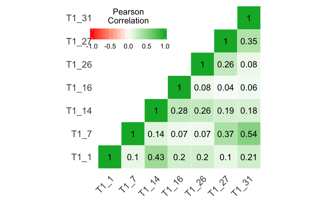
library(jmv)
reliability(
    data = westost,
    vars = c(
        "T1_2",
        "T1_8",
        "T1_15",
        "T1_23",
        "T1_29",
        "T1_32",
        "T1_35"),
    omegaScale = TRUE,
    meanScale = TRUE,
    sdScale = TRUE,
    corPlot = TRUE,
    alphaItems = TRUE,
    omegaItems = TRUE,
    meanItems = TRUE,
    sdItems = TRUE,
    itemRestCor = TRUE,
    revItems = "T1_2")
#>
#>  RELIABILITY ANALYSIS
#>
#>  Scale Reliability Statistics
#>  ──────────────────────────────────────────────────────────
#>             mean    sd       Cronbach's α    McDonald's ω
#>  ──────────────────────────────────────────────────────────
#>    scale    4.93    0.568           0.475           0.676
#>  ──────────────────────────────────────────────────────────
#>    Note. item 'T1_2' correlates negatively with the
#>    total scale and probably should be reversed
#>
#>
#>  Item Reliability Statistics
#>  ─────────────────────────────────────────────────────────────────────────────────────
#>               mean    sd       item-rest correlation    Cronbach's α    McDonald's ω
#>  ─────────────────────────────────────────────────────────────────────────────────────
#>    T1_2  ᵃ    2.80    1.262                   -0.606           0.762           0.783
#>    T1_8       5.50    1.098                    0.467           0.323           0.579
#>    T1_15      4.72    1.117                    0.441           0.334           0.625
#>    T1_23      4.55    1.487                    0.386           0.339           0.649
#>    T1_29      5.12    1.084                    0.450           0.333           0.621
#>    T1_32      5.77    1.000                    0.485           0.328           0.579
#>    T1_35      6.08    0.963                    0.451           0.348           0.589
#>  ─────────────────────────────────────────────────────────────────────────────────────
#>    ᵃ reverse scaled item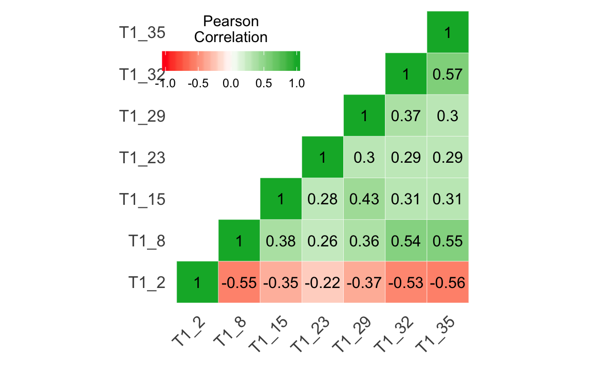
prop.table()uses as first argument a cross table as produced bytable(). Only if we use it with the pipe%>%we can use the unnamed value for the margin argument as presented above.