9 Functions
So far, we have neglected one of the most useful aspects of using R: the ability to automate our workflow and to let the computer do our work for us. Learning to write your own functions is one of the most important steps in this direction. Fortunately, R makes it very easy to create your own functions.
The basic idea of a function is that it takes one or more inputs, does something with these, and then returns an output. The inputs are called the function arguments, the code that does something with the arguments is called the function body, and the output is called the return value.
Suppose you want to write a function that squares a number and then adds 5. Let’s call the input argument x. First, we have to choose a name for our new function. We’ll call it square_add_five. Then, the function definition looks like this:
square_add_five <- function(x) {
    x^2 + 5
}
Once we have evaluated this code in the R console, we can call our function:
square_add_five(4)
#> [1] 21
or
square_add_five(x = 4)
#> [1] 21
The code x^2 + 5 is the function body. This takes the argument x, computes x^ and then adds 5 to the results. The result of this computation is returned, and can be assigned to a new variable:
result <- square_add_five(4)That’s the basic idea. Now we will take a closer look at how to translate a formula into R code, and then define a new function.
9.1 Skewness
In psychological research, we often measure response times. We have already looked at an example data set.
library(tidyverse)rt_wide <- read_csv("data/RTdata.csv")
#> Parsed with column specification:
#> cols(
#> ID = col_double(),
#> control = col_double(),
#> slow = col_double(),
#> fast = col_double()
#> )
rt_long <- rt_wide %>%
gather(key = condition, value = rt,
control, slow, fast, -ID) %>%
mutate(ID = factor(ID),
condition = factor(condition))rt_long %>%
ggplot(aes(x = rt)) +
geom_histogram(bins = 30, fill = "steelblue") +
facet_grid(condition ~ ID) +
xlab("Respone time") +
ylab("") +
theme_classic()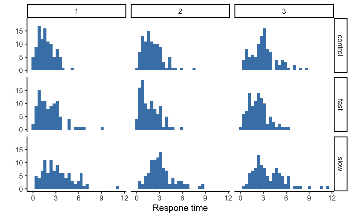
These data are right-skewed. We can calculate the skewness
\[ \mathrm{skewness} = \frac{\sum_{m=1}^{n}{(x_m - \bar{x})^3}} {n \cdot s_X^3} \]
\(x\) is a vector of observations with length \(n\), \(\bar{x}\) is its mean and \(s_X\) its empirical standard deviation \(s_X = \sqrt{\frac{1}{n}\sum_{m=1}^n{(x_m - \bar{x})^2}}\). For symmetrical distributions, the skewness is \(0\). For left-skewed distributions, the skewness is negative, for right-skewed distributions it’s positive. For RT data, we expect a value \(> 0\).
Unfortunately, there is no function in base R that can calculate this, but we can easily do so ourselves.
First, let’s translate the formula into R code. The formula can be simplified:
\[ \mathrm{skewness} = \frac{1}{n} \sum_{m=1}^{n} {z_m^3} \] with \[ z_m = \frac{x_m - \bar{x}} {s_X} \] To compute the skewness of a vector, we first standardize it, i.e. subtract its mean and divide by its standard deviation. Then we compute its third power and divide by \(n\).
Let’s generate some random numbers from a Gamma distribution. The Gamma distribition is only defined for positive numbers, and is right skewed.
set.seed(43772)
x1 <- 0.5 + rgamma(100, shape = 1.0, scale = .9)

ggplot(data = NULL, aes(x = x1)) +
    geom_histogram(bins = 30) + theme_classic()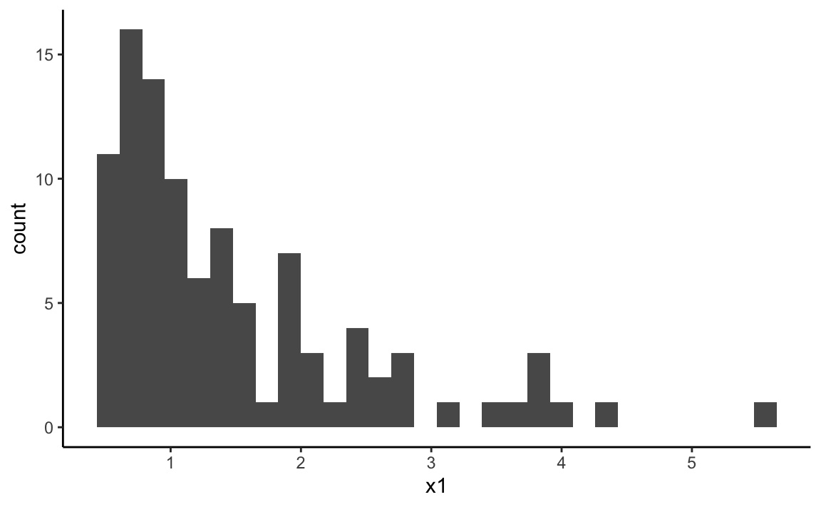
We need the lenght:
n <- length(x1)and the mean and standard deviation:
mean_x1 <- mean(x1)
sd_x1 <- sqrt(sum((x1 - mean_x1)^2) / (n))
Then we can standardize:
z1 <- (x1 - mean_x1) / sd_x1Now we can compute the skewness:
skewness <- sum(z1^3) / n
skewness
#> [1] 1.599983
The value we get is \(> 0\).
All the above steps in one code chunk:
n <- length(x1)
mean_x1 <- mean(x1)
sd_x1 <- sqrt(sum((x1 - mean_x1)^2) / (n))
z1 <- (x1 - mean_x1) / sd_x1
skewness <- sum(z1^3) / n
skewness
#> [1] 1.599983
So far so good, but what if we want to to this for another vector?
set.seed(43772)
x2 <- 0.6 + rgamma(120, shape = 0.8, scale = .95)

ggplot(data = NULL, aes(x = x2)) +
    geom_histogram(bins = 30) + theme_classic()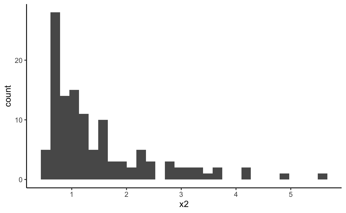
An obvious solution is to copy/paste our code from above, substituting x2 for x1.
n <- length(x2)
mean_x2 <- mean(x2)
sd_x2 <- sqrt(sum((x2 - mean_x2)^2) / (n))
z2 <- (x2 - mean_x2) / sd_x2
skewness <- sum(z2^3) / n
skewness
#> [1] 1.748647
This can be very error-prone.
Now we have a third vector:
set.seed(43772)
x3 <- 0.6 + rgamma(120, shape = 1.3, scale = 0.7)

ggplot(data = NULL, aes(x = x3)) +
    geom_histogram(bins = 30) + theme_classic()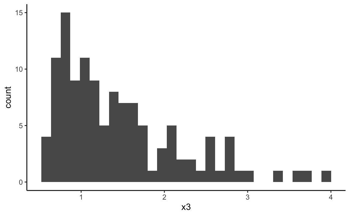
n <- length(x3)
mean_x3 <- mean(x3)
sd_x3 <- sqrt(sum((x2 - mean_x3)^2) / (n))
z3 <- (x3 - mean_x3) / sd_x3
skewness <- sum(z2^3) / n
skewness
#> [1] 1.748647
Can you spot two typos in the last code chunk?
It would be better to write a function. Then we only write the code once, and we can reuse it again and again without rewriting anything.
9.2 Defining a function
A function has a name and arguments:
function_name(arg1, arg2 = val2)The function function_name has two arguments, arg1 and arg2. Only arg2 has a default value. This means that arg1 is required.
Let’s give our skewness function the very descriptive name skewness. It will take one argument, x.
We use the function function() to define a new function:
skewness <- function(x) {
    # Code
}
Now we need the function body. This is the code between the curly braces {}. The last statement in the function body that is evaluated is automatically returned.
9.3 Skewness function
Now we are ready to define the skewness function:
skewness <- function(x) {

    n <- length(x)

    mean_x <- mean(x)
    sd_x <- sqrt(sum((x - mean_x)^2) / (n))

    # z-transform x and assign to z
    z <- (x - mean_x) / sd_x

    # this is not an evaluation, the result is assigned to skewness
    skewness <- sum(z^3) / n

    # we need to evaulate skewness
    # we could write
    # print(skewness)
    # or
    # return(skewness)
    skewness
}
You can send the code to the R console, or evaulate the function definition using a keyboard short cut.
Now you call the function:
skewness(x1)
#> [1] 1.599983
skewness(x2)
#> [1] 1.748647
And you call assign the returned value to another variable:
skew_x3 <- skewness(x3)
skew_x3
#> [1] 1.241044
9.4 Further examples
Let’s look at some more examples.
9.4.1 Multiplication
We want a function that takes two numbers as arguments, and multiplies both numbers. We will choose a default value of 1 for the second argument. This means that, unless we specify otherwise, the first arguments will be multiplied by \(1\), i.e. the function will return that number itself.
multiply <- function(x, k = 1) {
    k * x
}
# mit default value für k
value <- multiply(2)
value
#> [1] 2multiply(2, 3)
#> [1] 6
multiply(333, 43)
#> [1] 14319We can also call the function with named arguments:
multiply(x = 4, k = 2)
#> [1] 8
9.4.2 Standard deviation
In our next example, we will turn our standard devation code into a function. We also want to handle any missing values, so we will use the function na.omit().
standard_deviation <- function(x) {
    # remove NAs
    x <- na.omit(x)

    sqrt(sum((x - mean(x))^2) / (length(x)))
}standard_deviation(x1)
#> [1] 1.003002Does our function handle NAs correctly?
x <- rnorm(12)
# the first element of x is replaced by NA
x[1] <- NA
x
#>  [1]         NA -0.2933334 -1.1924669  3.4490925 -0.6391923  0.4956852
#> [7] -1.5414534 0.9317232 -2.2546778 -0.4523381 0.5655404 -1.2481360standard_deviation(x)
#> [1] 1.4782279.5 Exercise
9.5.1 Calculate skewness for RT data set
We can use our skewness() function just as any other function in R. This means that we can combine it with group_by() and summarise(), for example.
Let’s compute the skewness for each person in each condition in the rt_long data set.
rt_long %>%
    group_by(ID, condition) %>%
    summarise(skewness = skewness(rt))
#> # A tibble: 9 x 3
#> # Groups:   ID [3]
#>   ID    condition skewness
#>   <fct> <fct>        <dbl>
#> 1 1     control      0.559
#> 2 1     fast         1.45
#> 3 1     slow         0.987
#> 4 2     control      1.15
#> 5 2     fast         0.777
#> 6 2     slow         1.02
#> # … with 3 more rows
Why don’t we use the built-in
sd()function? The reason for this is that this function computes the sample standard deviation, by dividing by \(n-1\). We want to divive by \(n\), because we don’t want to estimate the population standard deviation. We are merely using the standard deviation descriptively.