8 Mean Comparisons
8.1 Comparison of a sample mean with a fixed (population) mean \((\mu_0)\) - one-Sample t test
Sometimes we want to compare a sample mean with a known population mean \((\mu_0)\) or some other fixed comparison value. For example, we would like to know whether the reported support by friends unt_freunde differs significantly from the midpoint of the 7-point-Likert scale \((\mu_0=4)\).
First, let’s create a data set that includes only the two support scales and some factors (for later analyses).
library(tidyverse)
load(file = "data/westost_scales.Rdata")
support <- westost_scales %>%
    select(ID,
           starts_with("unt"),
           westost, geschlecht,
           ends_with("_b"))

names(support)
#> [1] "ID"               "unt_eltern"       "unt_freunde"
#> [4] "westost"          "geschlecht"       "bildung_vater_b"
#> [7] "bildung_mutter_b"
The required function is t.test(). For the one-sample t test, we only need the following arguments (incl. default values): alternative = c("two.sided", "less", "greater"), mu = 0, and conf.level = .95.
TTest <- support$unt_freunde %>%
    t.test(alternative = 'two.sided',
           mu = 4,
           conf.level = .95)
TTest
#>
#>  One Sample t-test
#>
#> data:  .
#> t = 33.781, df = 284, p-value < 2.2e-16
#> alternative hypothesis: true mean is not equal to 4
#> 95 percent confidence interval:
#>  5.815396 6.040043
#> sample estimates:
#> mean of x
#>  5.927719
The output of the t.test() function is a list of the object class “htest” (hypothesis test).
typeof(TTest)
#> [1] "list"
attributes(TTest)
#> $names
#>  [1] "statistic"   "parameter"   "p.value"     "conf.int"    "estimate"
#>  [6] "null.value"  "stderr"      "alternative" "method"      "data.name"
#>
#> $class
#> [1] "htest"
The elements of this list can be selected individually. The (estimated) means can be obtained with:
TTest$estimate
#> mean of x
#>  5.927719
The p-value is returned with:
TTest$p.value
#> [1] 1.75588e-101
Degrees of freedom:
TTest$parameter
#>  df
#> 284
Confidence Interval:
TTest$conf.int
#> [1] 5.815396 6.040043
#> attr(,"conf.level")
#> [1] 0.95
The result shows that the sample mean (5.93) is signficantly different from the midpoint of the scale (=4) ($p=$0).
The example examined the non-directional alternative hypothesis \((H_1:\mu\neq\mu_0)\). For the directional alternative hypotheses \((H_1:\mu>\mu_0\) or \(H_1:\mu<\mu_0)\) specify alternative = "greater" or alternative = " less", respectively.
We can do a one-sample t test also with jmv:
library(jmv)
ttestOneS(
    data = support,
    vars = "unt_freunde",
    mann = FALSE,           # if TRUE -> Mann-Whitney U test
    testValue = 4,          # a number specifying the value of the null hypothesis
    hypothesis = 'dt',      # 'dt' (different to), 'gt' (greater than), 'lt' (less than)
    norm = TRUE,            # test for normality of the DV (Shapiro-Wilk test)
    meanDiff = TRUE,        # display estimated mean difference
    effectSize = TRUE,      # Cohen's d
    ci = TRUE,              # confidence interval of the mean
    ciWidth = 99,           # width of the confidence default: 95
    desc = TRUE)            # descriptive statistics
#>
#>  ONE SAMPLE T-TEST
#>
#>  One Sample T-Test
#>  ──────────────────────────────────────────────────────────────────────────────────────────────────────────────
#>                                  statistic    df     p         Mean difference    Lower    Upper    Cohen's d
#>  ──────────────────────────────────────────────────────────────────────────────────────────────────────────────
#>    unt_freunde    Student's t         33.8    284    < .001               1.93     1.78     2.08         2.00
#>  ──────────────────────────────────────────────────────────────────────────────────────────────────────────────
#>    Note. Hₐ population mean ≠ 4
#>
#>
#>  Test of Normality (Shapiro-Wilk)
#>  ──────────────────────────────────
#>                   W        p
#>  ──────────────────────────────────
#>    unt_freunde    0.892    < .001
#>  ──────────────────────────────────
#>    Note. A low p-value suggests
#>    a violation of the
#>    assumption of normality
#>
#>
#>  Descriptives
#>  ───────────────────────────────────────────────────────────
#>                   N      Mean    Median    SD       SE
#>  ───────────────────────────────────────────────────────────
#>    unt_freunde    285    5.93      6.00    0.963    0.0571
#>  ───────────────────────────────────────────────────────────
8.2 Comparison of two sample means
8.2.1 Two independent samples
Independent samples t test
For the t test for two independent samples we also use the function t.test(). In this case, the test variable and the factor are specified in the formula notation that is typical for R: Variable ~ Factor (\(\Rightarrow\) “Variable by Factor” = “test variable is predicted by factor” = “mean difference of the DV between the two levels of the factor”).
The data frame must be specified (data =) and we have to indicate whether the assumption of equal variances in the two groups holds: var.equal = FALSE / TRUE (FALSE is default). For var.equal = FALSE, the Welch Two Sample t test (heteroscedasticity corrected t test) is performed.
Again, the nature of the alternative hypothesis can be specified: If a directional alternative hypothesis is specified, the coding order of the factor levels must be taken into account. For example, we could hypothesize that girls will report a higher support received from friends (unt_freunde) than boys. Since in gender the order is "maennlich" "weiblich", the alternative hypothesis must be formulated as \(H_1:\mu_{Boys}<\mu_{Girls}\) (and not as \(\mu_{Girls}>\mu_{Boys}\)).
The required argument ‘alternative =’ less’ `refers to the format of the alternative hypothesis where a difference is compared to 0, in our case $ H_1:{boy}-{girl}<0$.
Let’s assume first that the population variances of unt_freunde are equal for boys and girls and carry out the “normal” t test:
levels(support$geschlecht)
#> [1] "männlich" "weiblich"
t.test(unt_freunde ~ geschlecht, alternative = "less",
       conf.level = .95,
       var.equal = TRUE,
       data = support)
#>
#>  Two Sample t-test
#>
#> data:  unt_freunde by geschlecht
#> t = -6.9351, df = 283, p-value = 1.379e-11
#> alternative hypothesis: true difference in means is less than 0
#> 95 percent confidence interval:
#>        -Inf -0.5598577
#> sample estimates:
#> mean in group männlich mean in group weiblich
#>               5.584868               6.319549
To check the homoscedasticity assumption, we now perform the Levene test with the function leveneTest() from the package car. In addition to the test variable and the factor, we have to specify which position measure (mean or median) we would like to use for the calculation of the deviations in the Levene test: for center = mean the (actual) Levene test is performed, forcenter = median (default) the Brown-Forsythe test, a more robust variant of the Levene test is performed.
library(car)
leveneTest(support$unt_freunde, support$geschlecht,
           center = median)
#> Levene's Test for Homogeneity of Variance (center = median)
#>        Df F value    Pr(>F)
#> group   1  11.987 0.0006185 ***
#>       283
#> ---
#> Signif. codes:  0 '***' 0.001 '**' 0.01 '*' 0.05 '.' 0.1 ' ' 1
Since the Levene test is significant, the null hypothesis of homoscedasticity has to be rejected. Therefore, we have to perform the t test again as a Welch test.
t.test(unt_freunde ~ geschlecht, alternative = "less",
       conf.level = .95, var.equal = FALSE,
       data = support)
#>
#>  Welch Two Sample t-test
#>
#> data:  unt_freunde by geschlecht
#> t = -7.0735, df = 275.37, p-value = 6.251e-12
#> alternative hypothesis: true difference in means is less than 0
#> 95 percent confidence interval:
#>        -Inf -0.5632619
#> sample estimates:
#> mean in group männlich mean in group weiblich
#>               5.584868               6.319549
Wilcoxon Rank Sum test for two independent samples (also known as Mann-Whitney U test)
A nonparametric alternative to the independent sample t test is the Wilcoxon rank sum test. It tests whether the average sum of the ranks (and thus the medians) of the two samples differ significantly from each other.
We use the function wilcox.exact() from the package exactRankTests, because unlike other functions this function calculates exact p-values even if there are ties.
As an example, let’s compare the medians of boys and girls with respect to the variable “Support by Parents” unt_eltern. Since we want to test the non-directional alternative hypothesis and alternative = "two.sided" is the default, we do not specify the argument. We also specify exact = FALSE because with a sample of n = 286 an exact test would require a lot of computation and also an exact test is not necessary with such a large n.
install.packages("exactRankTests")
library(exactRankTests)
wilcox.exact(unt_eltern ~ geschlecht,
             data = support,
             exact = FALSE)
#>
#>  Asymptotic Wilcoxon rank sum test
#>
#> data:  unt_eltern by geschlecht
#> W = 10380, p-value = 0.7036
#> alternative hypothesis: true mu is not equal to 0
In the results, the parameter W is actually the Mann-Whitney U.
As long as we do not need an exact test (with ties being present), we can also use the function wilcox.test() from the stats package (Base R). However, here we still have to specify correct = FALSE, otherwise an approximate test with continuity correction will be performed:
wilcox.test(unt_eltern ~ geschlecht,
            data = support,
            exact = FALSE,
            correct = FALSE)
#>
#>  Wilcoxon rank sum test
#>
#> data:  unt_eltern by geschlecht
#> W = 10380, p-value = 0.7036
#> alternative hypothesis: true location shift is not equal to 0
Here the t test for comparison:
t.test(unt_eltern ~ geschlecht, alternative = 'two.sided',
       conf.level = .95, var.equal = TRUE,
       data = support)
#>
#>  Two Sample t-test
#>
#> data:  unt_eltern by geschlecht
#> t = 1.303, df = 283, p-value = 0.1936
#> alternative hypothesis: true difference in means is not equal to 0
#> 95 percent confidence interval:
#>  -0.07868849  0.38688920
#> sample estimates:
#> mean in group männlich mean in group weiblich
#>                5.94415                5.79005
The exact Wilcoxon Rank Sum test is especially useful for very small samples:
x <- c(8.7, 4.5, 6.4, 8.7, 5.6, 6.2)
y <- c(8.6, 8.7, 9.8, 9.5, 8.3)
wilcox.exact(x, y, exact = TRUE)
#>
#>  Exact Wilcoxon rank sum test
#>
#> data:  x and y
#> W = 5, p-value = 0.08225
#> alternative hypothesis: true mu is not equal to 0
wilcox.test(x, y, exact = TRUE, correct = TRUE)
#> Warning in wilcox.test.default(x, y, exact = TRUE, correct = TRUE): cannot
#> compute exact p-value with ties
#>
#>  Wilcoxon rank sum test with continuity correction
#>
#> data:  x and y
#> W = 5, p-value = 0.08004
#> alternative hypothesis: true location shift is not equal to 0wilcox.exact(x, y, exact = FALSE)
#>
#> Asymptotic Wilcoxon rank sum test
#>
#> data: x and y
#> W = 5, p-value = 0.06539
#> alternative hypothesis: true mu is not equal to 0t.test(x, y, alternative = "two.sided",
conf.level = .95,
var.equal = TRUE)
#>
#> Two Sample t-test
#>
#> data: x and y
#> t = -2.8432, df = 9, p-value = 0.0193
#> alternative hypothesis: true difference in means is not equal to 0
#> 95 percent confidence interval:
#> -4.1240042 -0.4693291
#> sample estimates:
#> mean of x mean of y
#> 6.683333 8.980000In this example, the exact Wilcoxon Rank Sum test is not significant (p = 0.082), in the asymptotic test p- value approaches the significance criterion (p = 0.065), and the t test is significant (p = 0.019).
Tests for two independent samples with jmv
library(jmv)
ttestIS(
    data = support,
    vars = "unt_eltern",
    group = "geschlecht",
    welchs = TRUE,
    mann = TRUE,
    hypothesis = "oneGreater",  # 'different' (default),
                                # 'oneGreater'(group 1 greater than group 2)
                                # 'twoGreater'(group 2 greater than group 1)
    eqv = TRUE,                 #  Equality of Variances (Levene test)
    meanDiff = TRUE,
    effectSize = TRUE,
    ci = TRUE,
    ciWidth = 99,
    desc = TRUE)
#>
#>  INDEPENDENT SAMPLES T-TEST
#>
#>  Independent Samples T-Test
#>  ─────────────────────────────────────────────────────────────────────────────────────────────────────────────────────────────────
#>                                    statistic    df     p        Mean difference    SE difference    Lower     Upper    Cohen's d
#>  ─────────────────────────────────────────────────────────────────────────────────────────────────────────────────────────────────
#>    unt_eltern    Student's t            1.30    283    0.097              0.154            0.118    -0.123      Inf        0.155
#>                  Welch's t              1.28    249    0.100              0.154            0.120    -0.127      Inf        0.155
#>                  Mann-Whitney U         9854           0.352            6.64e-5                       -Inf    0.167        0.155
#>  ─────────────────────────────────────────────────────────────────────────────────────────────────────────────────────────────────
#>    Note. Hₐ männlich > weiblich
#>
#>
#>  ASSUMPTIONS
#>
#>  Test of Equality of Variances (Levene's)
#>  ────────────────────────────────────────
#>                  F       df    p
#>  ────────────────────────────────────────
#>    unt_eltern    9.08     1    0.003
#>  ────────────────────────────────────────
#>    Note. A low p-value suggests a
#>    violation of the assumption of
#>    equal variances
#>
#>
#>  Group Descriptives
#>  ──────────────────────────────────────────────────────────────────────
#>                  Group       N      Mean    Median    SD       SE
#>  ──────────────────────────────────────────────────────────────────────
#>    unt_eltern    männlich    151    5.94      6.17    0.869    0.0707
#>                  weiblich    134    5.79      6.17     1.12    0.0970
#>  ──────────────────────────────────────────────────────────────────────
8.2.2 Two dependent samples
Paired samples t Test
For this test we can we can again use the Base R function t.test().
As an example, we would like to test whether the extent of the support received from parents unt_parents differs from the extent of the support received from friends unt_freunde.
There are two options: Either we leave the dataset in wide format, where we have unt_eltern and unt_freunde as two variables (columns) in the dataset next to each other.
In this case, the data assignment for the t.test () function is not done using the formula notation but by specifying the two variables to be compared. The only difference to the t test for independent samples is that we specify the option paired = TRUE (default:paired = FALSE), reflecting the dependence of the data in the two samples/variables.
t.test(support$unt_eltern, support$unt_freunde,
       alternative = "two.sided",
       conf.level = .95,
       paired = TRUE)
#>
#>  Paired t-test
#>
#> data:  support$unt_eltern and support$unt_freunde
#> t = -0.73804, df = 283, p-value = 0.4611
#> alternative hypothesis: true difference in means is not equal to 0
#> 95 percent confidence interval:
#>  -0.21046776  0.09567902
#> sample estimates:
#> mean of the differences
#>             -0.05739437
The second option is to convert the dataset from wide to long, taking into account that parents and friends are actually two levels of a factor, that is the source of the support (unt_quelle). The measured variable is support (for both factor levels). (The items that underlie unt_parents andunt_freunde are the same, they only differ in the reference given to parents or friends.)
library(stringr)
sup_long <- support %>%
    drop_na(unt_eltern, unt_freunde) %>%
    select(ID, unt_eltern, unt_freunde) %>%
    gather(key = unt_quelle, value = unterstuetzung, -ID) %>%
    mutate(unt_quelle = str_replace(unt_quelle, ".*_", "")) %>%     # unt_ entfernen
mutate(unt_quelle = factor(unt_quelle))library(ggplot2)
sup_long %>%
ggplot(aes(x = unt_quelle, y = unterstuetzung, fill = unt_quelle)) +
geom_boxplot() +
theme_classic()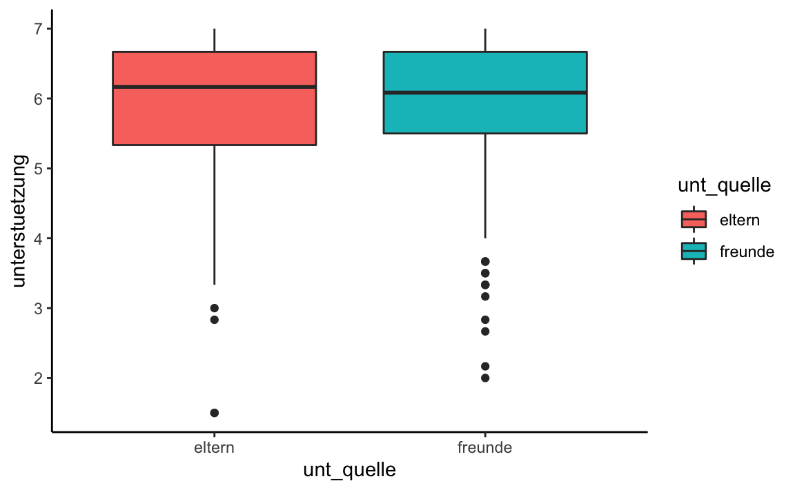
sup_long %>%
    group_by(unt_quelle) %>%
    summarize(mean = mean(unterstuetzung, na.rm = TRUE),
              N = length(unterstuetzung))
#> # A tibble: 2 x 3
#>   unt_quelle  mean     N
#>   <fct>      <dbl> <int>
#> 1 eltern      5.87   284
#> 2 freunde 5.93 284t.test(unterstuetzung ~ unt_quelle,
alternative = "two.sided",
conf.level = .95,
paired = TRUE,
data = sup_long)
#>
#> Paired t-test
#>
#> data: unterstuetzung by unt_quelle
#> t = -0.73804, df = 283, p-value = 0.4611
#> alternative hypothesis: true difference in means is not equal to 0
#> 95 percent confidence interval:
#> -0.21046776 0.09567902
#> sample estimates:
#> mean of the differences
#> -0.05739437Wilcoxon Signed Rank test
A nonparametric alternative to the paired sample t-test is the Wilcoxon Signed Rank test. This test checks whether the mean rank sums of the negative and positive differences of the two variables are significantly different. Thus, as in the paired sample t-test, a difference variable is created, then ranks are assigned for the absolute values of the differences, and then the mean rank sums are determined separately according to the sign of the respective difference score.
For this test there is also an exact and an approximate option.
Again we use the function wilcox.exact() from the package exactRankTests, as it can calculate exact p-values, even in the presence of ties. The only difference to the Wilcoxon Rank Sum test is that we need to use the argument paired = TRUE. Again, we do not need the exact test here due to the large sample size. The test statistic V refers to the rank sum of the positive differences.
wilcox.exact(support$unt_eltern, support$unt_freunde,
             alternative = "two.sided",
             paired = TRUE,
             exact = FALSE)
#>
#>  Asymptotic Wilcoxon signed rank test
#>
#> data:  support$unt_eltern and support$unt_freunde
#> V = 16477, p-value = 0.9335
#> alternative hypothesis: true mu is not equal to 0
Or using the long dataset and formula notation:
wilcox.exact(unterstuetzung ~ unt_quelle,
             alternative = "two.sided",
             paired = TRUE,
             exact = FALSE,
             data = sup_long)
#>
#>  Asymptotic Wilcoxon signed rank test
#>
#> data:  unterstuetzung by unt_quelle
#> V = 16477, p-value = 0.9335
#> alternative hypothesis: true mu is not equal to 0
Paired samples tests with jmv
library(jmv)
ttestPS(
    data = support,
    pairs = list(
        list(
            i1 = "unt_eltern",
            i2 = "unt_freunde")),
    wilcoxon = TRUE,
    meanDiff = TRUE,
    effectSize = TRUE,
    ci = TRUE,
    desc = TRUE)
#>
#>  PAIRED SAMPLES T-TEST
#>
#>  Paired Samples T-Test
#>  ──────────────────────────────────────────────────────────────────────────────────────────────────────────────────────────────────────────────
#>                                                statistic    df     p        Mean difference    SE difference    Lower     Upper     Cohen's d
#>  ──────────────────────────────────────────────────────────────────────────────────────────────────────────────────────────────────────────────
#>    unt_eltern    unt_freunde    Student's t       -0.738    283    0.461            -0.0574           0.0778    -0.210    0.0957      -0.0438
#>                                 Wilcoxon W         16477           0.934           -5.29e-5           0.0778    -0.167     0.167      -0.0438
#>  ──────────────────────────────────────────────────────────────────────────────────────────────────────────────────────────────────────────────
#>
#>
#>  Descriptives
#>  ───────────────────────────────────────────────────────────
#>                   N      Mean    Median    SD       SE
#>  ───────────────────────────────────────────────────────────
#>    unt_eltern     284    5.87      6.17    0.999    0.0593
#>    unt_freunde    284    5.93      6.08    0.963    0.0571
#>  ───────────────────────────────────────────────────────────
8.3 Mean comparisons of more than two samples
8.3.1 Multiple independent samples
One-way Analysis of Variance
We perform a one-way ANOVA with the grade average (Schnitt) as a dependent variable and and the level of education of the father (bildung_vater) as a factor (independent variable). The null hypothesis is that the means of the grade average do not differ between groups of adolescents whose fathers have different levels of education.
First, we create a data set grades containing only the variables ID,Schnitt, bildung_vater and geschlecht (for later analysis) and remove all persons with missing values.
grades <- westost_scales %>%
    select(ID, Schnitt, bildung_vater, geschlecht) %>%
    drop_na()
grades
#> # A tibble: 264 x 4
#>   ID    Schnitt bildung_vater                       geschlecht
#>   <fct>   <dbl> <fct>                               <fct>
#> 1 2           4 Fachabitur, Abitur                  männlich
#> 2 14          4 Realschulabschluss (mittlere Reife) männlich
#> 3 15          4 Realschulabschluss (mittlere Reife) männlich
#> 4 17          4 Realschulabschluss (mittlere Reife) männlich
#> 5 18          4 Fachabitur, Abitur                  männlich
#> 6 19          4 Hauptschulabschluss oder niedriger  männlich
#> # … with 258 more rows
Since the labels of the factor levels are very long and this is inconvenient for displaying results, let us relabel the factor levels:
table(grades$bildung_vater)
#>
#>            Hauptschulabschluss oder niedriger
#>                                            41
#>           Realschulabschluss (mittlere Reife)
#>                                            93
#>                            Fachabitur, Abitur
#>                                            39
#> Fachhochschulabschluss, Universitätsabschluss
#>                                            91
levels(grades$bildung_vater) <-  c("Hauptschule", "Realschule", "Abitur", "Hochschule")

# since there is a problem with the umlauts for this online script we change
# this here as well:
levels(grades$geschlecht) <-  c("maennlich", "weiblich")
table(grades$bildung_vater)
#>
#> Hauptschule  Realschule      Abitur  Hochschule
#>          41          93          39          91
Before performing the ANOVA we can get descriptive statistics (means and standard deviations) using our well-known dplyr function summarize():
grades %>%
    group_by(bildung_vater) %>%
    summarize(mean = round(mean(Schnitt, na.rm = TRUE), 2),
              sd = round(sd(Schnitt, na.rm = TRUE), 3),
              N = length(Schnitt))
#> # A tibble: 4 x 4
#>   bildung_vater  mean    sd     N
#>   <fct>         <dbl> <dbl> <int>
#> 1 Hauptschule    4.05 0.669    41
#> 2 Realschule     4.38 0.655    93
#> 3 Abitur         4.5  0.653    39
#> 4 Hochschule     4.69 0.683    91
Thus, descriptively, higher educational levels of the father are related to a higher overall grade average of students.
The standard deviations of the DV seem to be similar across groups. To check the assumption of homogeneity of variances we can use the leveneTest() function.
library(car)
leveneTest(grades$Schnitt, grades$bildung_vater,
           center = median)
#> Levene's Test for Homogeneity of Variance (center = median)
#>        Df F value Pr(>F)
#> group   3  0.4906 0.6891
#>       260
The result of the Levene test confirms that there are no significant differences in the variances. Thus, we can assume homscedasticity.
Now we can compute the ANOVA using the aov() function, save the output in a results object and then use the summary() function to access the output.
In addition, we want to use the TukeyHSD function to get all pairwise comparisons (adjusted confidence intervals and Tukey p-values).
Anova.model1 <- aov(Schnitt ~ bildung_vater, data = grades)
summary(Anova.model1)
#>                Df Sum Sq Mean Sq F value   Pr(>F)
#> bildung_vater   3  12.36   4.120   9.272 7.58e-06 ***
#> Residuals     260 115.53   0.444
#> ---
#> Signif. codes:  0 '***' 0.001 '**' 0.01 '*' 0.05 '.' 0.1 ' ' 1
TukeyHSD(Anova.model1, ordered = TRUE)
#>   Tukey multiple comparisons of means
#>     95% family-wise confidence level
#>     factor levels have been ordered
#>
#> Fit: aov(formula = Schnitt ~ bildung_vater, data = grades)
#>
#> $bildung_vater
#>                             diff          lwr       upr     p adj
#> Realschule-Hauptschule 0.3269866  0.003864173 0.6501091 0.0461134
#> Abitur-Hauptschule     0.4437774  0.058237843 0.8293169 0.0167437
#> Hochschule-Hauptschule 0.6397481  0.315540988 0.9639551 0.0000039
#> Abitur-Realschule      0.1167907 -0.212031612 0.4456131 0.7950495
#> Hochschule-Realschule  0.3127614  0.058608643 0.5669142 0.0088548
#> Hochschule-Abitur      0.1959707 -0.133917530 0.5258589 0.4174570
Alternatively, we can use the ANOVA function ezANOVA() from the package ez:
install.packages("ez")
With this function it is necessary to specify an ID variable using the argument wid = ID. The function white.adjust = FALSE is used to suppress the implementation of a heteroscedasticity-adjusted ANOVA. Since the Levene test is provided in the output, it is possible to adjust this option if necessary.
library(ez)
ezANOVA(grades, dv = Schnitt, wid = ID,
        between = bildung_vater,
        white.adjust = FALSE,
        detailed = TRUE)
#> Coefficient covariances computed by hccm()
#> $ANOVA
#>          Effect DFn DFd     SSn      SSd        F            p p<.05
#> 1 bildung_vater   3 260 12.3607 115.5329 9.272342 7.575436e-06     *
#>         ges
#> 1 0.0966483
#>
#> $`Levene's Test for Homogeneity of Variance`
#>   DFn DFd       SSn      SSd         F         p p<.05
#> 1   3 260 0.4063397 71.78362 0.4905869 0.6891123
In addition to the TukeyHSD() function that can be applied to the aov() outcome object, there is another way to obtain post-hoc pairwise comparisons: pairwise.t.test() from the stats package. Among others, the methods p.adjust.method = c("bonferroni", "holm") are available. The pairwise.t.test() function works independently of the ANOVA procedure (i.e., it simply performs pairwise comparisons without an overall test).
pairwise.t.test(grades$Schnitt, grades$bildung_vater,
                p.adjust.method = "holm", data = grades)
#>
#>  Pairwise comparisons using t tests with pooled SD
#>
#> data:  grades$Schnitt and grades$bildung_vater
#>
#>            Hauptschule Realschule Abitur
#> Realschule 0.0282      -          -
#> Abitur     0.0128      0.3593     -
#> Hochschule 3.9e-06     0.0082     0.2515
#>
#> P value adjustment method: holm
Kruskal-Wallis test (H test)
The H test is a non-parametric alternative to the one-way analysis of variance. It is an extension of the Wilcoxon rank sum test to multiple samples. The Kruskal-Wallis test is usually carried out asymptotically, since an exact test requires a lot of computing power - at least with larger samples - and is usually not necessary.
First, let’s get the medians using dplyr:
grades %>%
    group_by(bildung_vater) %>%
    summarise(median = median(Schnitt))
#> # A tibble: 4 x 2
#>   bildung_vater median
#>   <fct>          <dbl>
#> 1 Hauptschule      4
#> 2 Realschule       4
#> 3 Abitur           4.6
#> 4 Hochschule       5
For comparison we also use the tapply() function for displaying the medians:
tapply(grades$Schnitt, grades$bildung_vater,
       median, na.rm = TRUE)
#> Hauptschule  Realschule      Abitur  Hochschule
#>         4.0         4.0         4.6         5.0
Then the Kruskal-Wallis H test can be obtained by:
kruskal.test(Schnitt ~ bildung_vater, data = grades)
#>
#>  Kruskal-Wallis rank sum test
#>
#> data:  Schnitt by bildung_vater
#> Kruskal-Wallis chi-squared = 29.008, df = 3, p-value = 2.231e-06
A box-plot could be nice to illustrate the median difference:
grades %>%
    ggplot(aes(x = bildung_vater, y = Schnitt)) +
    geom_boxplot() +
    geom_jitter() +
    xlab("Bildung des Vaters") +
    theme_classic()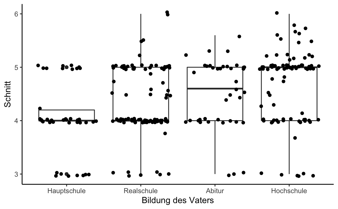
Several post-hoc pairwise comparison methods are provided by the PMCMRplus package.
install.packages("PMCMRplus")
library(PMCMRplus)
kwAllPairsNemenyiTest(x = grades$Schnitt,
                             g = grades$bildung_vater,
                             dist = "Tukey")
#>
#>  Pairwise comparisons using Tukey-Kramer-Nemenyi all-pairs test with Tukey-Dist approximation
#> data: grades$Schnitt and grades$bildung_vater
#>            Hauptschule Realschule Abitur
#> Realschule 0.1663      -          -
#> Abitur     0.0375      0.6818     -
#> Hochschule 8.6e-06     0.0024     0.3740
#>
#> P value adjustment method: single-step
#> alternative hypothesis: two.sided
kwAllPairsConoverTest(x = grades$Schnitt,
                             g = grades$bildung_vater,
                             p.adjust.method = "holm")
#>
#>  Pairwise comparisons using Conover's all-pairs test
#> data: grades$Schnitt and grades$bildung_vater
#>            Hauptschule Realschule Abitur
#> Realschule 0.07161     -          -
#> Abitur     0.01381     0.22085    -
#> Hochschule 1.4e-06     0.00064    0.15454
#>
#> P value adjustment method: holm
kwAllPairsDunnTest(x = grades$Schnitt,
                             g = grades$bildung_vater,
                             p.adjust.method = "holm")
#>
#>  Pairwise comparisons using Dunn's all-pairs test
#>
#> data: grades$Schnitt and grades$bildung_vater
#>            Hauptschule Realschule Abitur
#> Realschule 0.0933      -          -
#> Abitur     0.0205      0.2443     -
#> Hochschule 2.8e-06     0.0011     0.1849
#>
#> P value adjustment method: holm
#> alternative hypothesis: two.sided
The Kruskal-Wallis test can also be performed by anovaNP() from the jmv package:
library(jmv)
anovaNP(grades, deps = "Schnitt", group = "bildung_vater",
      pairs = TRUE)
#>
#>  ONE-WAY ANOVA (NON-PARAMETRIC)
#>
#>  Kruskal-Wallis
#>  ───────────────────────────────────
#>               χ²      df    p
#>  ───────────────────────────────────
#>    Schnitt    29.0     3    < .001
#>  ───────────────────────────────────
#>
#>
#>  DWASS-STEEL-CRITCHLOW-FLIGNER PAIRWISE COMPARISONS
#>
#>  Pairwise comparisons - Schnitt
#>  ───────────────────────────────────────────────
#>                                 W       p
#>  ───────────────────────────────────────────────
#>    Hauptschule    Realschule    3.38     0.017
#>    Hauptschule    Abitur        4.16     0.003
#>    Hauptschule    Hochschule    6.76    < .001
#>    Realschule     Abitur        1.75     0.216
#>    Realschule     Hochschule    5.31    < .001
#>    Abitur         Hochschule    2.57     0.069
#>  ───────────────────────────────────────────────
Factorial ANOVA
We would like to investigate whether the two factors educational level of the father (bildung_vater) and gender (geschlecht) have an impact on adolescents’ grade average and how these two factors may interact.
First let’s get descriptive statistics with dplyr:
 grades %>%
    group_by(bildung_vater, geschlecht) %>%
    summarize(mean = round(mean(Schnitt, na.rm = TRUE), 2),
             sd = round(sd(Schnitt, na.rm = TRUE), 3),
              var = round(var(Schnitt, na.rm = TRUE), 3),
              N = length(Schnitt))
#> # A tibble: 8 x 6
#> # Groups:   bildung_vater [?]
#>   bildung_vater geschlecht  mean    sd   var     N
#>   <fct>         <fct>      <dbl> <dbl> <dbl> <int>
#> 1 Hauptschule   maennlich   3.86 0.640 0.409    22
#> 2 Hauptschule   weiblich    4.27 0.651 0.423    19
#> 3 Realschule    maennlich   4.13 0.626 0.392    48
#> 4 Realschule    weiblich    4.65 0.578 0.334    45
#> 5 Abitur        maennlich   4.39 0.694 0.481    21
#> 6 Abitur        weiblich    4.63 0.595 0.354    18
#> # ... with 2 more rows
 grades %>%
    group_by(geschlecht) %>%
    summarize(mean = round(mean(Schnitt, na.rm = TRUE), 2),
              sd = round(sd(Schnitt, na.rm = TRUE), 3),
              var = round(var(Schnitt, na.rm = TRUE), 3),
              N = length(Schnitt))
#> # A tibble: 2 x 5
#>   geschlecht  mean    sd   var     N
#>   <fct>      <dbl> <dbl> <dbl> <int>
#> 1 maennlich   4.29 0.723 0.522   145
#> 2 weiblich    4.65 0.612 0.375   119
Then we carry out the Levene test to check whether homogenous variances can be assumed:
library(car)
leveneTest(grades$Schnitt ~ grades$bildung_vater * grades$geschlecht,
           center = median)
#> Levene's Test for Homogeneity of Variance (center = median)
#>        Df F value Pr(>F)
#> group   7  1.1221 0.3495
#>       256
First, we perform the two-factorial analysis of variance using the traditional aov() method:
Anova.model2 <- aov(Schnitt ~ bildung_vater * geschlecht, data = grades)
Anova(Anova.model2, type = 3)
#> Anova Table (Type III tests)
#>
#> Response: Schnitt
#>                          Sum Sq  Df  F value    Pr(>F)
#> (Intercept)              328.41   1 799.1587 < 2.2e-16 ***
#> bildung_vater              9.90   3   8.0335 3.891e-05 ***
#> geschlecht                 1.71   1   4.1714   0.04214 *
#> bildung_vater:geschlecht   0.85   3   0.6875   0.56041
#> Residuals                105.20 256
#> ---
#> Signif. codes:  0 '***' 0.001 '**' 0.01 '*' 0.05 '.' 0.1 ' ' 1
A complete model (with all the main effects and interactions) can be specified like this: FactorA * FactorB. This is equivalent to FactorA + FactorB + FactorA:FactorB. So if you only want the two main effects without the interaction effect, you connect the factors with + instead of *.
It is important that we request the summary of the ANOVA outcome object with the function Anova() from the car package. This is the only way we can get Type II or Type III sums of squares (type = 2 ortype = 3). The default and only option for summary() are Type I sums of squares that return a sequential partialization of all effects.
\(~\)
With ezANOVA() we obtain the same result:
library(ez)
ezANOVA(grades, dv = Schnitt, wid = ID,
        between = bildung_vater * geschlecht,
        white.adjust = FALSE,
        type = 3)
#> Coefficient covariances computed by hccm()
#> $ANOVA
#>                     Effect DFn DFd          F            p p<.05
#> 2            bildung_vater   3 256 10.3151356 1.965388e-06     *
#> 3               geschlecht   1 256 17.8024414 3.404755e-05     *
#> 4 bildung_vater:geschlecht   3 256  0.6874928 5.604118e-01
#>           ges
#> 2 0.107844231
#> 3 0.065019294
#> 4 0.007992167
#>
#> $`Levene's Test for Homogeneity of Variance`
#>   DFn DFd      SSn    SSd        F         p p<.05
#> 1   7 256 2.070602 67.483 1.122133 0.3494653
8.3.2 Multiple dependent samples
(One-Way) Repeated Measures ANOVA
As an example, let’s look at the fictitious study on “Honeymoon or Hangover” (using an example from the book by [Budischewski & Kriens, 2012] (https://www.beltz.de/fachmedien/psychologie/books/produkt_produktdetails/4144-aufgabensammlung_statistik.html). In this study, n = 10 employees from two companies (n = 5 each) were interviewed at the beginning of their employment (Anfang) as well as at two further measurement points (Drei Monate, Sechs Monate) regarding their job satisfaction (Arbeitszufriedenheit). The hypothesis was that employees are very satisfied at the beginning, as they enthusiastically approach the new task (“honeymoon”), then due to the heavy workload at a new entry a phase of lesser satisfaction follows (“hangover”) before the level of satisfaction levels off (here after six months). In general, we ask about the differences in the mean values of job satisfaction over time. We start with only one company (company 1).
For the Repeated Measures ANOVA we have to create long format dataset first. Let’s import the SPSS dataset honeymoon_hangover_2companies.sav and then use the gather() function from tidyr to convert from wide to long.
library(haven)
Honeymoon <- read_sav("data/honeymoon_hangover_2Firmen.sav")
Honeymoon$ID <- as.factor(Honeymoon$ID)
Honeymoon$Firma <- as.factor(Honeymoon$Firma)
Honeymoon
#> # A tibble: 10 x 5
#>   ID    Firma Anfang Drei_Monate Sechs_Monate
#>   <fct> <fct>  <dbl>       <dbl>        <dbl>
#> 1 1     1          9           4            5
#> 2 2     1          9           4            8
#> 3 3     1          9           7           14
#> 4 4     1         10           9            5
#> 5 5     1          8           1            3
#> 6 6     2         10          10           10
#> # … with 4 more rows
Honeymoon_long <- Honeymoon %>%
gather(key = Messzeitpunkt, value = Arbeitszufriedenheit,
-Firma, -ID) %>%
mutate(Messzeitpunkt = factor(Messzeitpunkt)) %>%
arrange(Firma, ID)
Honeymoon_long
#> # A tibble: 30 x 4
#> ID Firma Messzeitpunkt Arbeitszufriedenheit
#> <fct> <fct> <fct> <dbl>
#> 1 1 1 Anfang 9
#> 2 1 1 Drei_Monate 4
#> 3 1 1 Sechs_Monate 5
#> 4 2 1 Anfang 9
#> 5 2 1 Drei_Monate 4
#> 6 2 1 Sechs_Monate 8
#> # … with 24 more rowsLet’s get the means of the DV:
Honeymoon_long %>%
    group_by(Firma, Messzeitpunkt) %>%
    summarise(Bedingungsmittelwert = mean(Arbeitszufriedenheit))
#> # A tibble: 6 x 3
#> # Groups:   Firma [2]
#>   Firma Messzeitpunkt Bedingungsmittelwert
#>   <fct> <fct>                        <dbl>
#> 1 1     Anfang                         9
#> 2 1     Drei_Monate                    5
#> 3 1     Sechs_Monate                   7
#> 4 2     Anfang                        10
#> 5 2     Drei_Monate                   10.8
#> 6 2     Sechs_Monate                  11
First, we only want to examine the development of job satisfaction in the first company:
# select company 1
Honeymoon_long_F1 <- Honeymoon_long %>%
    filter(Firma == 1)

# means for company 1
Honeymoon_long_F1 %>%
    group_by(Messzeitpunkt) %>%
    summarise(Bedingungsmittelwert = mean(Arbeitszufriedenheit))
#> # A tibble: 3 x 2
#>   Messzeitpunkt Bedingungsmittelwert
#>   <fct>                        <dbl>
#> 1 Anfang                           9
#> 2 Drei_Monate                      5
#> 3 Sechs_Monate                     7
We get the repeated measures ANOVA by defining the variable Messzeitpunkt as a within-factor in ezANOVA():
library(ez)
ezANOVA(Honeymoon_long_F1, dv = Arbeitszufriedenheit,
        wid = ID, within = Messzeitpunkt,
        detailed = TRUE)
#> $ANOVA
#>          Effect DFn DFd SSn SSd         F          p p<.05       ges
#> 1   (Intercept)   1   4 735  60 49.000000 0.00219213     * 0.8657244
#> 2 Messzeitpunkt   2   8  40  54  2.962963 0.10890896       0.2597403
#>
#> $`Mauchly's Test for Sphericity`
#>          Effect         W        p p<.05
#> 2 Messzeitpunkt 0.6872428 0.569725
#>
#> $`Sphericity Corrections`
#>          Effect       GGe     p[GG] p[GG]<.05      HFe    p[HF] p[HF]<.05
#> 2 Messzeitpunkt 0.7617555 0.1308327           1.134177 0.108909
Since the Mauchly test is not significant, we can maintain the null hypothesis of a spherical variance-covariance matrix (sphericity assumption) and therefore do not need to make any corrections. The effect of the factor ‘time of measurement’ is not significant. Our very small sample of n = 5 is associated with a very low statistical power, though.
Because of the low power of the Mauchly test we could still apply the corrections according to Greenhouse Geisser-\(\epsilon\) (GGe) or Huynh-Feldt-$$ (HFe): also the p[GG] and p[HF] are both non-significant.
\(~\)
Post-hoc tests can be obtained using the pairwise.t.test() from stats, where we have to specify paired = TRUE. Here we use both the uncorrected pairwise comparisons (p.adjust.method = "none") and the Bonferroni-Holm corrected comparisons (p.adjust.method = "holm").
pairwise.t.test(Honeymoon_long_F1$Arbeitszufriedenheit,
                Honeymoon_long_F1$Messzeitpunkt,
                p.adjust.method = "none",
                paired = TRUE,
                data = Honeymoon_long_F1)
#>
#>  Pairwise comparisons using paired t tests
#>
#> data:  Honeymoon_long_F1$Arbeitszufriedenheit and Honeymoon_long_F1$Messzeitpunkt
#>
#>              Anfang Drei_Monate
#> Drei_Monate  0.022  -
#> Sechs_Monate 0.351  0.333
#>
#> P value adjustment method: none

pairwise.t.test(Honeymoon_long_F1$Arbeitszufriedenheit,
                Honeymoon_long_F1$Messzeitpunkt,
                p.adjust.method = "holm",
                paired = TRUE,
                data = Honeymoon_long_F1)
#>
#>  Pairwise comparisons using paired t tests
#>
#> data:  Honeymoon_long_F1$Arbeitszufriedenheit and Honeymoon_long_F1$Messzeitpunkt
#>
#>              Anfang Drei_Monate
#> Drei_Monate  0.065  -
#> Sechs_Monate 0.665  0.665
#>
#> P value adjustment method: holm
We can do the RM ANOVA also with jmv. In jmv we need a wide dataset again since the philosophy of jmv and the associated GUI [jamovi] (https://www.jamovi.org) is to emulate the functionality of SPSS!
So let us select company 1 from the Honeymooon_wide dataset:
Honeymoon_wide_F1 <- Honeymoon %>%
    filter(Firma == 1)
The syntax of the anovaRM() function is quite complicated. It would be much easier to define the model terms of a RM ANOVA in a long data set:
anovaRM(
    data = Honeymoon_wide_F1,
    rm = list(                   # Definition of RM factor / factor levels
        list(
            label = "Messzeitpunkt",
            levels = c("Anfang", "Drei_Monate", "Sechs_Monate"))),
    rmCells = list(              # Assignment of the DV (measure)
        list(                    # to the cells (factor levels)
            measure = "Anfang",
            cell = "Anfang"),
        list(
            measure = "Drei_Monate",
            cell = "Drei_Monate"),
        list(
            measure = "Sechs_Monate",
            cell = "Sechs_Monate")),
    rmTerms = list(              # Calling those RM model terms that should
        "Messzeitpunkt"),        # be used in the current model
    effectSize = c("eta", "omega"),
    spherTests = TRUE,
    spherCorr = c("none", "GG", "HF"))
#>
#>  REPEATED MEASURES ANOVA
#>
#>  Within Subjects Effects
#>  ──────────────────────────────────────────────────────────────────────────────────────────────────────────────────────
#>                     Sphericity Correction    Sum of Squares    df      Mean Square    F       p        η²       ω²
#>  ──────────────────────────────────────────────────────────────────────────────────────────────────────────────────────
#>    Messzeitpunkt    None                               40.0       2          20.00    2.96    0.109    0.260    0.165
#>                     Greenhouse-Geisser                 40.0    1.52          26.26    2.96    0.131    0.260    0.165
#>                     Huynh-Feldt                        40.0    2.00          20.00    2.96    0.109    0.260    0.165
#>
#>    Residual         None                               54.0       8           6.75
#>                     Greenhouse-Geisser                 54.0    6.09           8.86
#>                     Huynh-Feldt                        54.0    8.00           6.75
#>  ──────────────────────────────────────────────────────────────────────────────────────────────────────────────────────
#>    Note. Type 3 Sums of Squares
#>
#>
#>  Between Subjects Effects
#>  ───────────────────────────────────────────────────────────────────────────────────
#>                Sum of Squares    df    Mean Square    F    p        η²       ω²
#>  ───────────────────────────────────────────────────────────────────────────────────
#>    Residual              60.0     4           15.0
#>  ───────────────────────────────────────────────────────────────────────────────────
#>    Note. Type 3 Sums of Squares
#>
#>
#>  ASSUMPTIONS
#>
#>  Tests of Sphericity
#>  ──────────────────────────────────────────────────────────────────────────────────
#>                     Mauchly's W    p        Greenhouse-Geisser ε    Huynh-Feldt ε
#>  ──────────────────────────────────────────────────────────────────────────────────
#>    Messzeitpunkt          0.687    0.570                   0.762             1.00
#>  ──────────────────────────────────────────────────────────────────────────────────
Friedman Repeated Measures ANOVA for Rank Data
The Friedman test is a non-parametric alternative to the repeated measures ANOVA. It is an extension of the Wilcoxon signed rank test to multiple connected samples. The Friedman test is usually performed asymptotically, because an exact test requires quite some computing power (with large samples).
Unfortunately, the Friedman test does not work with ID being a factor, so we have to convert ID into a numeric vector first.
Honeymoon_long_F1$ID <- as.numeric(Honeymoon_long_F1$ID)
friedman.test(Arbeitszufriedenheit ~ Messzeitpunkt | ID,
              data = Honeymoon_long_F1)
#>
#>  Friedman rank sum test
#>
#> data:  Arbeitszufriedenheit and Messzeitpunkt and ID
#> Friedman chi-squared = 6.4, df = 2, p-value = 0.04076
Let’s look at the median differences using box plot:
Honeymoon_long_F1 %>%
    ggplot(aes(x = Messzeitpunkt, y = Arbeitszufriedenheit)) +
    geom_boxplot() +
    geom_point() +
    theme_classic()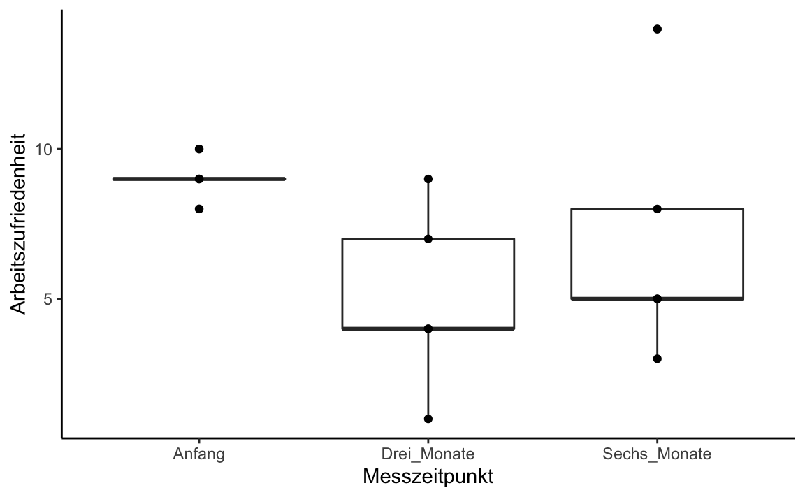
\(~\)
Post-hoc pairwise comparisons can be obtained again with PMCMRplus:
library(PMCMRplus)
frdAllPairsNemenyiTest(y = Honeymoon_long_F1$Arbeitszufriedenheit,
                              groups  = Honeymoon_long_F1$Messzeitpunkt,
                              blocks = Honeymoon_long_F1$ID,
                              data = Honeymoon_long_F1)
#>
#>  Pairwise comparisons using Nemenyi-Wilcoxon-Wilcox all-pairs test for a two-way balanced complete block design
#> data: Honeymoon_long_F1$Arbeitszufriedenheit , Honeymoon_long_F1$Messzeitpunkt and Honeymoon_long_F1$ID
#>              Anfang Drei_Monate
#> Drei_Monate  0.031  -
#> Sechs_Monate 0.415  0.415
#>
#> P value adjustment method: single-step

frdAllPairsConoverTest(y = Honeymoon_long_F1$Arbeitszufriedenheit,
                              groups  = Honeymoon_long_F1$Messzeitpunkt,
                              blocks = Honeymoon_long_F1$ID,
                              data = Honeymoon_long_F1,
                       p.adjust.method = "holm")
#>
#>  Pairwise comparisons using Conover's all-pairs test for a two-way balanced complete block design
#>
#> data: Honeymoon_long_F1$Arbeitszufriedenheit , Honeymoon_long_F1$Messzeitpunkt and Honeymoon_long_F1$ID
#>              Anfang Drei_Monate
#> Drei_Monate  0.11   -
#> Sechs_Monate 0.48   0.48
#>
#> P value adjustment method: holm
frdAllPairsExactTest(y = Honeymoon_long_F1$Arbeitszufriedenheit,
                              groups  = Honeymoon_long_F1$Messzeitpunkt,
                              blocks = Honeymoon_long_F1$ID,
                              data = Honeymoon_long_F1,
                       p.adjust.method = "holm")
#>
#>  Pairwise comparisons using Eisinga, Heskes, Pelzer & Te Grotenhuis all-pairs test with exact p-values for a two-way balanced complete block design
#>
#> data: Honeymoon_long_F1$Arbeitszufriedenheit , Honeymoon_long_F1$Messzeitpunkt and Honeymoon_long_F1$ID
#>              Anfang Drei_Monate
#> Drei_Monate  0.039  -
#> Sechs_Monate 0.565  0.565
#>
#> P value adjustment method: holm
durbinAllPairsTest(y = Honeymoon_long_F1$Arbeitszufriedenheit,
                              groups  = Honeymoon_long_F1$Messzeitpunkt,
                              blocks = Honeymoon_long_F1$ID,
                              data = Honeymoon_long_F1,
                       p.adjust.method = "none")
#>
#>  Pairwise comparisons using Durbin's all-pairs test for a two-way balanced incomplete block design
#> data: Honeymoon_long_F1$Arbeitszufriedenheit, Honeymoon_long_F1$Messzeitpunkt and Honeymoon_long_F1$ID
#>              Anfang Drei_Monate
#> Drei_Monate  0.0055 -
#> Sechs_Monate 0.0961 0.0961
#>
#> P value adjustment method: none
The Friedman test is also in jmv. For anovaRMNP() we need the wide data set again:
library(jmv)
anovaRMNP(Honeymoon_wide_F1,
          measures = c("Anfang", "Drei_Monate", "Sechs_Monate"),
          pairs = TRUE)
#>
#>  REPEATED MEASURES ANOVA (NON-PARAMETRIC)
#>
#>  Friedman
#>  ───────────────────────
#>    χ²      df    p
#>  ───────────────────────
#>    6.40     2    0.041
#>  ───────────────────────
#>
#>
#>  Pairwise Comparisons (Durbin-Conover)
#>  ──────────────────────────────────────────────────────────
#>                                        Statistic    p
#>  ──────────────────────────────────────────────────────────
#>    Anfang         -    Drei_Monate          3.77    0.005
#>    Anfang         -    Sechs_Monate         1.89    0.096
#>    Drei_Monate    -    Sechs_Monate         1.89    0.096
#>  ──────────────────────────────────────────────────────────
Mixed (within-between) design ANOVA
We now want to compare the development of job satisfaction across the two companies.
Honeymoon_long %>%
    group_by(Firma, Messzeitpunkt) %>%
    summarise(Bedingungsmittelwert = mean(Arbeitszufriedenheit))
#> # A tibble: 6 x 3
#> # Groups:   Firma [2]
#>   Firma Messzeitpunkt Bedingungsmittelwert
#>   <fct> <fct>                        <dbl>
#> 1 1     Anfang                         9
#> 2 1     Drei_Monate                    5
#> 3 1     Sechs_Monate                   7
#> 4 2     Anfang                        10
#> 5 2     Drei_Monate                   10.8
#> 6 2     Sechs_Monate                  11
The mixed-design ANOVA is obtained by defining the variable Messzeitpunkt as within-factor and Firma as between-factor in ezANOVA():
library(ez)
ezANOVA(Honeymoon_long, dv = Arbeitszufriedenheit,
        wid = ID, within = Messzeitpunkt,
        between = Firma, detailed = TRUE)
#> $ANOVA
#>                Effect DFn DFd    SSn  SSd          F            p p<.05
#> 1         (Intercept)   1   8 2323.2 87.6 212.164384 4.837731e-07     *
#> 2               Firma   1   8   97.2 87.6   8.876712 1.761704e-02     *
#> 3       Messzeitpunkt   2  16   13.4 57.2   1.874126 1.856652e-01
#> 4 Firma:Messzeitpunkt   2  16   29.4 57.2   4.111888 3.622639e-02     *
#>          ges
#> 1 0.94132901
#> 2 0.40165289
#> 3 0.08470291
#> 4 0.16877153
#>
#> $`Mauchly's Test for Sphericity`
#>                Effect         W         p p<.05
#> 3       Messzeitpunkt 0.7122598 0.3049541
#> 4 Firma:Messzeitpunkt 0.7122598 0.3049541
#>
#> $`Sphericity Corrections`
#>                Effect       GGe      p[GG] p[GG]<.05       HFe      p[HF]
#> 3       Messzeitpunkt 0.7765541 0.19689735           0.9289728 0.18928790
#> 4 Firma:Messzeitpunkt 0.7765541 0.05071043           0.9289728 0.04029652
#>   p[HF]<.05
#> 3
#> 4         *
To do this in jmv we need the wide data set again (Honeymoon, including both companies).
We get the mixed-design ANOVA by adding the arguments bs = 'Firma' (definition of the between subjects factor) and bsTerms = "Firma" to the previous code for the RM ANOVA. The latter argument indicates which of the factors listed under bs should be used in the model. The interaction effect between the bs factor and the rm factor is included automatically.
anovaRM(
    data = Honeymoon,
    rm = list(                   # Definition of RM factor / factor levels
        list(
            label = "Messzeitpunkt",
            levels = c("Anfang", "Drei_Monate", "Sechs_Monate"))),
    rmCells = list(              # Assignment of the DV (measure)
        list(                    # to the cells (factor levels)
            measure = "Anfang",
            cell = "Anfang"),
        list(
            measure = "Drei_Monate",
            cell = "Drei_Monate"),
        list(
            measure = "Sechs_Monate",
            cell = "Sechs_Monate")),
    rmTerms = list(              # Calling those RM model terms that should
        "Messzeitpunkt"),        # be used in the current model
    bs = "Firma",                # Definition of between factor
    bsTerms = list(              # Calling those "between" model terms that should
        "Firma"),                # be used in the current model
    effectSize = c("eta", "omega"),
    spherTests = TRUE,
    spherCorr = c("none", "GG", "HF"))
#>
#>  REPEATED MEASURES ANOVA
#>
#>  Within Subjects Effects
#>  ─────────────────────────────────────────────────────────────────────────────────────────────────────────────────────────────
#>                           Sphericity Correction    Sum of Squares    df       Mean Square    F       p        η²       ω²
#>  ─────────────────────────────────────────────────────────────────────────────────────────────────────────────────────────────
#>    Messzeitpunkt          None                               13.4        2           6.70    1.87    0.186    0.047    0.022
#>                           Greenhouse-Geisser                 13.4     1.55           8.63    1.87    0.197    0.047    0.022
#>                           Huynh-Feldt                        13.4     1.86           7.21    1.87    0.189    0.047    0.022
#>
#>    Messzeitpunkt:Firma    None                               29.4        2          14.70    4.11    0.036    0.103    0.077
#>                           Greenhouse-Geisser                 29.4     1.55          18.93    4.11    0.051    0.103    0.077
#>                           Huynh-Feldt                        29.4     1.86          15.82    4.11    0.040    0.103    0.077
#>
#>    Residual               None                               57.2       16           3.58
#>                           Greenhouse-Geisser                 57.2    12.42           4.60
#>                           Huynh-Feldt                        57.2    14.86           3.85
#>  ─────────────────────────────────────────────────────────────────────────────────────────────────────────────────────────────
#>    Note. Type 3 Sums of Squares
#>
#>
#>  Between Subjects Effects
#>  ──────────────────────────────────────────────────────────────────────────────────────
#>                Sum of Squares    df    Mean Square    F       p        η²       ω²
#>  ──────────────────────────────────────────────────────────────────────────────────────
#>    Firma                 97.2     1           97.2    8.88    0.018    0.341    0.292
#>    Residual              87.6     8           10.9
#>  ──────────────────────────────────────────────────────────────────────────────────────
#>    Note. Type 3 Sums of Squares
#>
#>
#>  ASSUMPTIONS
#>
#>  Tests of Sphericity
#>  ──────────────────────────────────────────────────────────────────────────────────
#>                     Mauchly's W    p        Greenhouse-Geisser ε    Huynh-Feldt ε
#>  ──────────────────────────────────────────────────────────────────────────────────
#>    Messzeitpunkt          0.712    0.305                   0.777            0.929
#>  ──────────────────────────────────────────────────────────────────────────────────
We use the formula notation here, but it is also possible to specify two vectors/variables that contain the values of the two groups (see below).