12 Bootstrap
12.1 Setup
pacman::p_load(boot,
               tidyverse,
               lme4)
12.2 Basics
Bootstrap is a term describing different resampling methods.
Resampling generally refers to the method creating a new set of data by randomly drawing data points out of an existing dataset. Bootstrapping is not the only application of a resampling method. Other popular applications are permutation tests, see this blogpost for a short introduction.
Bootstrapping is most often used to compute estimate uncertainty and bias. Uncertainty can be captured in a confidence interval. We can also compute a bias estimate, i.e. the estimated difference of our observed statistic and the expected value.
Lets say we have a sample of grades of students for the last statistics exam:
grades <- c(sample(seq(4,6,by = .5), size = 20, replace = TRUE),
            sample(seq(1,3.5,by = .5), size = 5, replace = TRUE))
hist(grades) 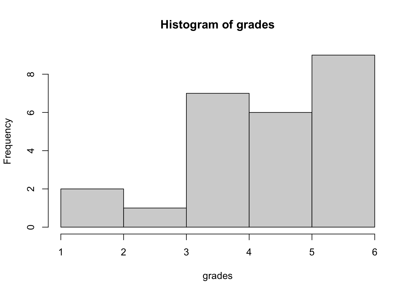
We would like to estimate the mean of the population (all students). We can do this with bootstrap to include uncertainty about the distribution of the mean in the population.
Instead of assuming a specific distribution of grades and constructing a CI around our estimate, we sample from the empirical distribution.
Our grades vector corresponds perfectly to this empirical distribution.
Hence, we can sample directly from the grades vector.
N times.
plot(ecdf(grades), verticals = TRUE)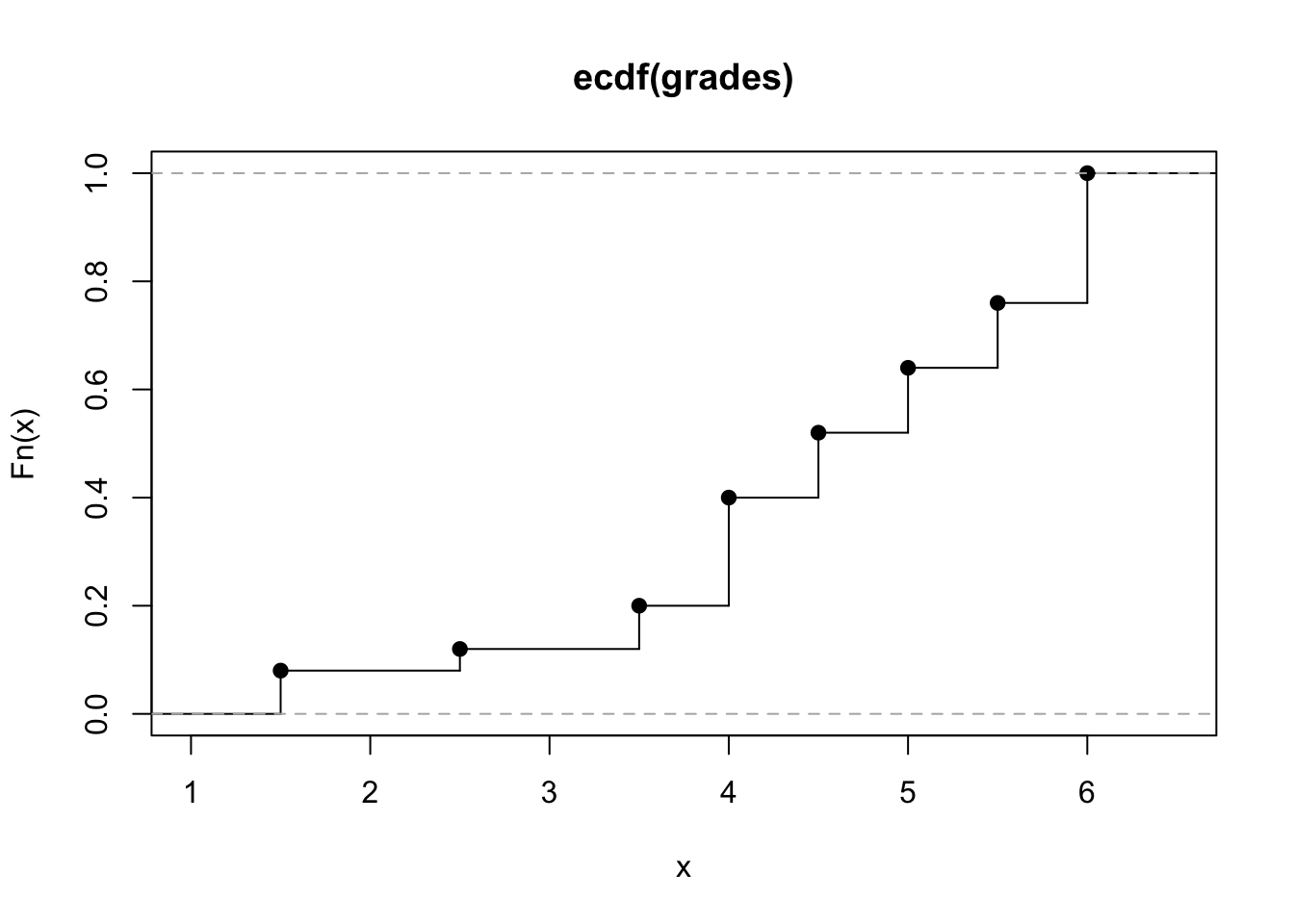
The following animations are taken from here. The data does not correspond to our example but it visualizes the process very well.
GIF of univariate bootstrap
We have to allow replacement as not allowing it would mean that each draw would depend on all draws before. This means that some entries will likely be drawn more than once. If there will be duplicated entries, there must be some entries of the original dataframe missing as well. How many unique data points (or rows / entries) would we expect for a bootstrap sample? Naturally, we can simulate this: Let’s say, for n = 100.
nn <- 1:100
mean(replicate(n = 1000, length(unique(sample(nn, replace = TRUE)))))
## [1] 63.408Looks like our resampled dataframe will contain about 63 or 64 unique entries for n = 100. We can offer also an analytic solution, dependent on n.
rep_fn <- function(n){
  p <- 1/n # probability of drawing a specific row at each draw
  # 1-p is then the probability of not drawing a row
  # (1-p)^n is the probability of not drawing a specific row for n draws.
  # This corresponds to the percentage of rows which were not drawn in a bootstrap sample.
  1-(1-p)^n # All other rows will be drawn.
}

rep_fn(100)
## [1] 0.6339677n_vec <- seq(1, 15)
p_vec <- rep_fn(n_vec)
plot(p_vec, type = "l", ylim = c(0,1), xlab = "n", ylab = "expected proportion of unique rows")
# analytic limit of rep_fn (as n -> inf):
abline(h = 1-1/exp(1), col = "red")
title(sub = "Expected proportion of unique rows drawn in bootstrap for specific sample size")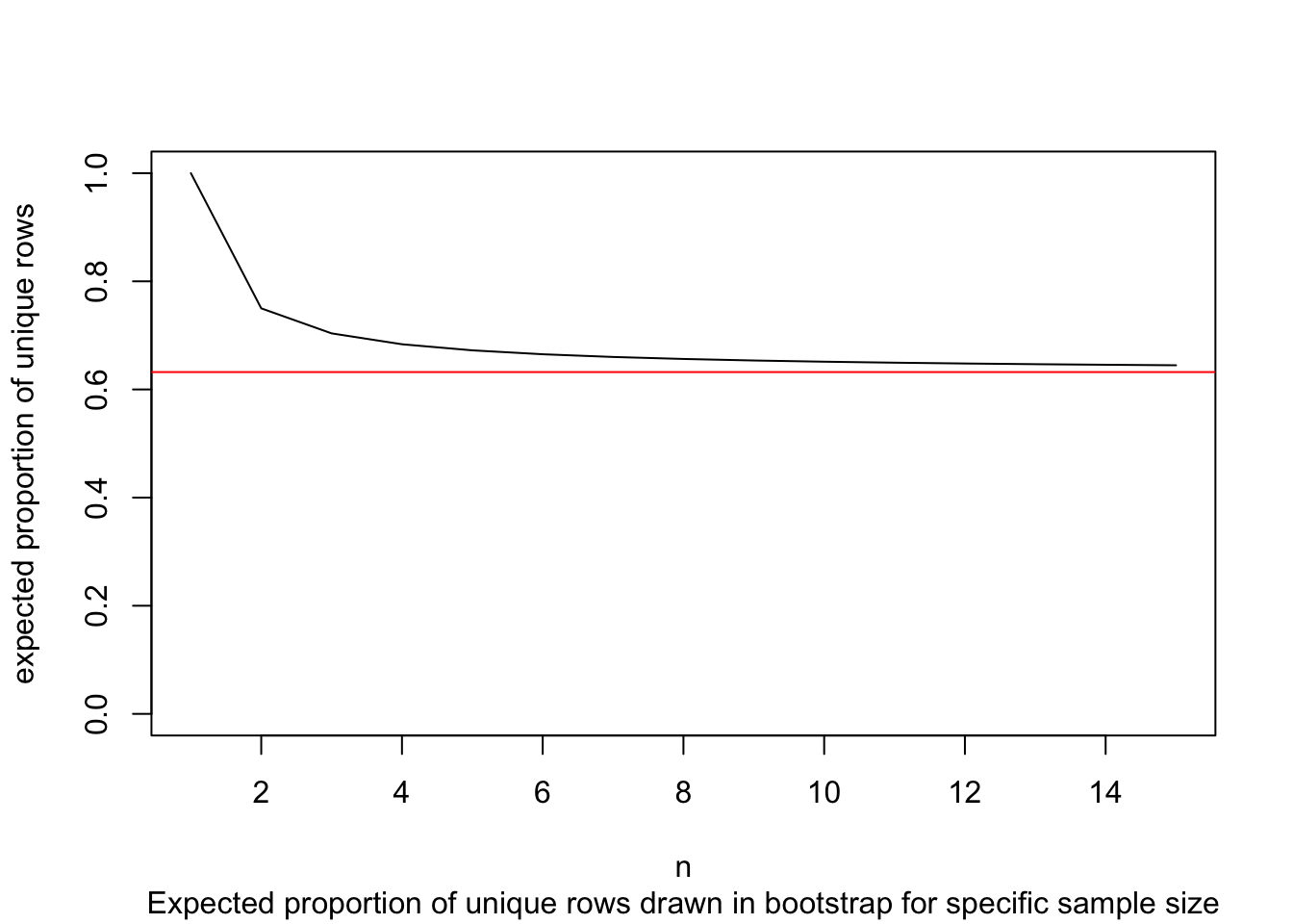
12.3 Non-parametric vs semi-parametric vs parametric bootstrap
When we have a linear model such as this:
\[Y=\beta_{0}+\beta_{1}X_{1}+\beta_{2}X_2+\varepsilon_{i}\] Where \(\varepsilon \sim \mathcal{N}(\theta, \sigma^2)\)
There are different ways to compute a bootstrap.
So, according to our model specification our errors are normally distributed. Lets say we have a sample of size 100 generated from such a model with \(\beta_0 = 5\), \(\beta_1 = 3\) and \(\beta_2 = .4\). The error variance is specified as \(\varepsilon \sim \mathcal{N}(\theta = 0, \sigma^2 = 5)\)
set.seed(6134346)
# parameters
n <- 100
b0 <- 5
b1 <- 3
b2 <- .4
var <- 5


# data simulation
X1 <- sample(0:1, size = n, replace = TRUE)
X2 <- rnorm(n)
Y <- b0 + b1 * X1 + b2 * X2 + rnorm(n, sd = sqrt(var))
We then have a dataset randomly generated according to our model specifications.
original <- data.frame(ID = 1:length(Y), X1, X2, Y)

ggplot(data = original, aes(y = Y, x = X2, col = as_factor(X1))) +
  geom_point() +
  theme_classic()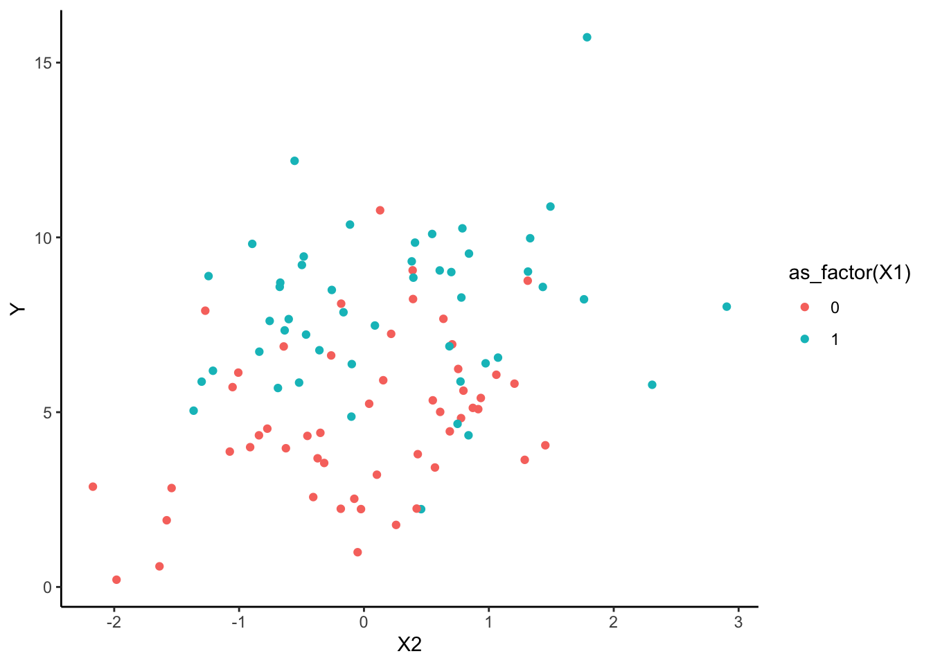
Of course, you usually don’t know the true parameter of the data generating process. Instead, you have to estimate them.
coef(lm(Y ~ X1 + X2, data = original))## (Intercept) X1 X2
## 4.7953170 3.0049359 0.6664353We get parameter estimates, and could compute corresponding confidence intervals based on the t-statistic. But we could also compute confidence intervals based on bootstrap samples.
12.3.1 Bootstrap resample functions by hand
In the non-parametric bootstrap we simply re-sample the data-points and then re-estimate the model parameters:
GIF of univariate bootstrap
We can create a function to do exactly this:
nonpara.boot <- function(){
  size <- nrow(original)
  temp.data <- original[sample(1:size, size, replace = TRUE), ]

  # re-estimate parameters:
  coef(lm(Y ~ X1 + X2, data = temp.data))[3]
}
In a semi-parametric bootstrap, we use the model prediction on the original predictor variables and randomly reassign the residuals:
semipara.boot <- function(){
  size <- nrow(original)
  original.model <- lm(Y ~ X1 + X2, data = original)
  residuals <- resid(original.model)
  model.pred <- predict(original.model)

  temp.data <- original
  temp.data$Y <- model.pred + residuals[sample(1:size, size, replace = TRUE)]

  # re-estimate parameters:
  coef(lm(Y ~ X1 + X2, data = temp.data))[3]
  }
The parametric bootstrap relies on our assumption that the residuals are normally distributed, and resamples from the estimated error distribution.
parametric.boot <- function(){
  size <- nrow(original)
  original.model <- lm(Y ~ X1 + X2, data = original)
  residuals <- rnorm(size, mean = 0, sd = summary(original.model)$sigma)
  model.pred <- predict(original.model)

  temp.data <- original
  temp.data$Y <- model.pred + residuals[sample(1:size, size, replace = TRUE)]

  # re-estimate parameters:
  coef(lm(Y ~ X1 + X2, data = temp.data))[3]
  }
12.3.2 Resampling
We can now use the functions created above to draw a specified number of bootstrap samples of our parameter estimates.
nboot <- 1000

nonpara.samples <- replicate(nboot, nonpara.boot())

semipara.samples <- replicate(nboot, semipara.boot())

para.samples <- replicate(nboot, parametric.boot())


samples.dat <- data.frame(id = 1:nboot,
                          nonpara = nonpara.samples,
                          semipara = semipara.samples,
                          parametric = para.samples) %>%
  pivot_longer(
    cols = c("nonpara", "semipara", "parametric"),
    names_to = "type",
    values_to = "statistic"
  )
Now we can plot the bootstrapped statistics:
pacman::p_load(patchwork) # allows stitching plots together

histo <- ggplot(data = samples.dat,
       aes(x = statistic, fill = type)) +
  geom_histogram() +
  facet_wrap(~type) +
  theme_classic()


densi <- ggplot(data = samples.dat,
       aes(x = statistic, color = type)) +
  geom_density() +
  theme_classic() +
  theme(legend.position = "none")

histo / densi + plot_layout(guides = "collect")
## `stat_bin()` using `bins = 30`. Pick better value with `binwidth`.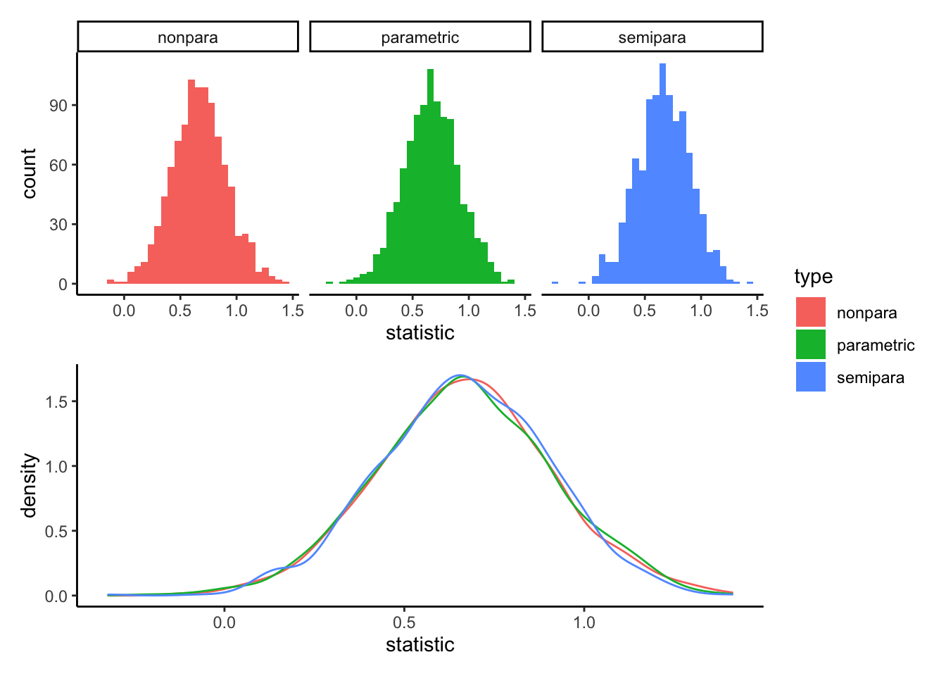
12.4 Boot package (and extension)
12.4.1 Bootstrap resampling
To bootstrap with the boot() function we still need to create a function for statistic sampling, still dependent on the type of bootstrap we want to conduct.
Again, the function differs between parametric and non-parametric bootstrap, but both are possible using the boot() function.
Importantly, we have to write a function that accepts two inputs: the original data, and a vector of indices which facilitates the data shuffling (i.e. the choice of rows to sample from the data).
The boot() function is designed to accept multiple parameter estimates as output of the bootstrap function, so we can simultaneously bootstrap all model parameters.
boot.nonpara.fn <- function(data, indices){
  temp.data <- data[indices, ]
  # re-estimate parameters:
  coef(lm(Y ~ X1 + X2, data = temp.data))
  }


booted.nonpara.est <- boot::boot(data = original,
                                 statistic = boot.nonpara.fn,
                                 R = nboot)

booted.nonpara.est
##
## ORDINARY NONPARAMETRIC BOOTSTRAP
##
##
## Call:
## boot::boot(data = original, statistic = boot.nonpara.fn, R = nboot)
##
##
## Bootstrap Statistics :
## original bias std. error
## t1* 4.7953170 0.003583439 0.2880788
## t2* 3.0049359 0.009609618 0.4154549
## t3* 0.6664353 0.004120620 0.2527025We can look at the vector of bootstrapped estimates at object$t
head(booted.nonpara.est$t)## [,1] [,2] [,3]
## [1,] 4.722757 3.582802 0.6037329
## [2,] 4.842129 2.778300 0.6872599
## [3,] 4.926578 2.805035 0.9604704
## [4,] 5.044137 2.609505 0.6259701
## [5,] 4.664711 3.463633 1.4127219
## [6,] 4.798308 3.447769 0.4478153For a parametric bootstrap we need to work a little more.
We need to set up a function that computes the parameters given a data set.
This function is very similar to the function above (booted.nonpara.fn()).
But, it does not need to have a second argument, and does not need resampling of the rows:
boot.para.fn <- function(data){
  # reestimate parameters
    coef(lm(Y ~ X1 + X2, data = data))
}
We need not shuffle the rows in the statistic funtion because the data used in that function is created using another function we need to set up: A data creation function. This function needs as input the original data and the (MLE) parameter estimates
# the data creation function.
# the model consists of 4 estimates, three beta coefficients and the estimated error variance.
boot.data.fn <- function(data, theta){
  data$Y <-theta[1] +  theta[2] * data$X1 + theta[3] * data$X2  + # original model prediction
    rnorm(n = nrow(data), mean = 0, sd = theta[4]) # residuals
  # this could also be solved using the predict function
  #data$Y <- predict(lm(Y ~ X1 + X2, data = original)) + rnorm(n = nrow(data), mean = 0, sd = theta[4])

  return(data)
}
Where theta is:
theta <- c(coef(fit <- lm(Y ~ X1 + X2, data = original)), sigma(fit))And the boot() function is specified like this:
booted.para.est <- boot::boot(data = original,
                              statistic = boot.para.fn,
                              R = nboot,
                              sim = "parametric",
                              ran.gen = boot.data.fn,
                              mle = theta)

booted.para.est
##
## PARAMETRIC BOOTSTRAP
##
##
## Call:
## boot::boot(data = original, statistic = boot.para.fn, R = nboot,
## sim = "parametric", ran.gen = boot.data.fn, mle = theta)
##
##
## Bootstrap Statistics :
## original bias std. error
## t1* 4.7953170 0.010092838 0.3066339
## t2* 3.0049359 -0.003027481 0.4485276
## t3* 0.6664353 -0.009693141 0.230998212.4.2 Bootstrap confidence intervals
We will have a look at two types of bootstrap confidence intervals (CI). But there are more ways to constuct CI’s using bootstraped estimates.
We can compute CI’s using the boot.ci() function of the boot package.
As input, it takes the output of the boot() function above.
The function allows us to specify the type of CI we wish to compute.
Here, we will introduce the two most common CI types.
Normal CI
This CI relies on the assumption that the bootstrap parameter samples are normally distributed.
We can check this by applying the generic plot() function to the output of the boot() function.
plot(booted.para.est, index = 3)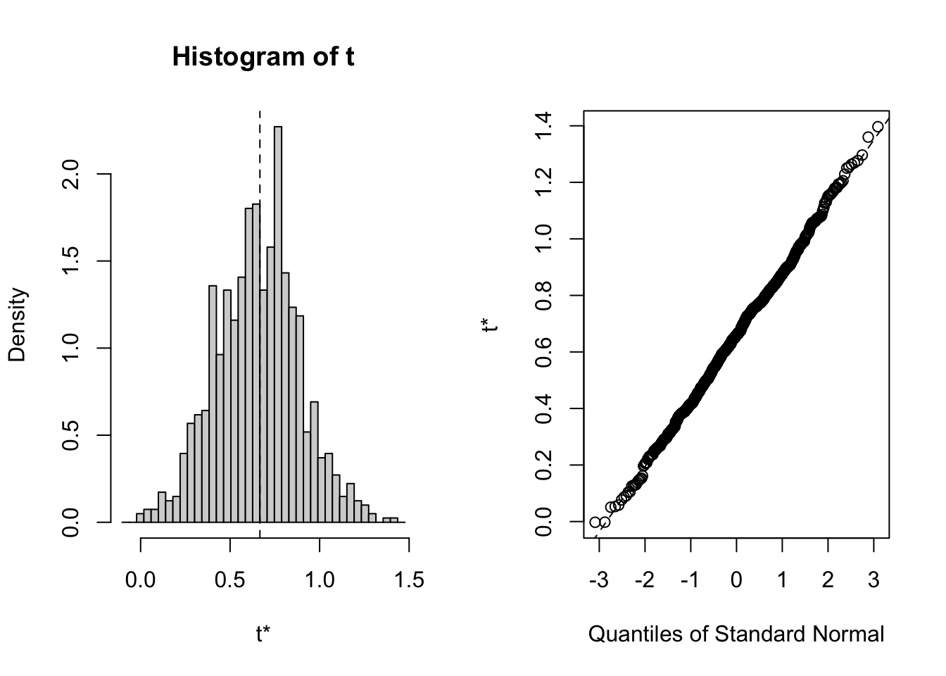
Seems appropriate.
We can then specify type = "norm" in boot.ci() to get a symmetric CI around
booted.para.ci <- boot.ci(boot.out = booted.para.est,
        conf = .95,
        type = "norm",
        index = 3) # indicates which parameter we are interested in

booted.para.ci
## BOOTSTRAP CONFIDENCE INTERVAL CALCULATIONS
## Based on 1000 bootstrap replicates
##
## CALL :
## boot.ci(boot.out = booted.para.est, conf = 0.95, type = "norm",
## index = 3)
##
## Intervals :
## Level Normal
## 95% ( 0.2234, 1.1289 )
## Calculations and Intervals on Original ScaleConfirm by hand:
# lower bound
booted.para.est$t0[3]  - # original estimate
  (mean(booted.para.est$t[, 3]) - booted.para.est$t0[3]) - # bias
  qnorm(p =  .975) * # .975 quantile (ca. 1.96)
    sd(booted.para.est$t[, 3]) # standard error
## X2
## 0.2233803# upper bound
booted.para.est$t0[3] - # original estimate
(mean(booted.para.est$t[, 3]) - booted.para.est$t0[3]) + # bias
qnorm(p = .975) * # .975 quantile (ca. 1.96)
sd(booted.para.est$t[, 3]) # standard error ## X2
## 1.128877Percentile CI
“perc”: Percentile, we look at the empirical distribution of the bootstrapped estimates and chose as lower limit of the ci the .025% percentile, and for the upper limit the .975 percentile.
booted.nonpara.ci <- boot.ci(boot.out = booted.nonpara.est,
        conf = .95,
        type = "perc",
        index = 3) # indicates which parameter we are interested in

booted.nonpara.ci
## BOOTSTRAP CONFIDENCE INTERVAL CALCULATIONS
## Based on 1000 bootstrap replicates
##
## CALL :
## boot.ci(boot.out = booted.nonpara.est, conf = 0.95, type = "perc",
## index = 3)
##
## Intervals :
## Level Percentile
## 95% ( 0.1739, 1.1610 )
## Calculations and Intervals on Original ScaleSomething similar but not equitailed we can do easily by just getting the quantiles of the bootstrapped estimates:
# lower bound
quantile(booted.nonpara.est$t[,3], probs = c(.025, .975))
## 2.5% 97.5%
## 0.1857002 1.159878012.4.3 Mixed effects models
Mixed effects models can be bootstrapped using the bootMer() function supplied by the lme4 package.
Again, we need to supply a statistic function.
However, the function only takes one input, namely a fitted merMod object (a mixed effects model fitted by lmer() or glmer()).
To show how it works, we again look at the salary example:
df <- read_csv(
  url("https://raw.githubusercontent.com/methodenlehre/data/master/salary-data2.csv")) %>%
  mutate(company = as.factor(company),
         sector = as.factor(sector),
         id = as_factor(1:nrow(.)))
## Rows: 600 Columns: 4## ── Column specification ────────────────────────────────────────────────────────
## Delimiter: ","
## chr (2): company, sector
## dbl (2): experience, salary##
## ℹ Use `spec()` to retrieve the full column specification for this data.
## ℹ Specify the column types or set `show_col_types = FALSE` to quiet this message.And fit the model:
random.intercept.model <-  lmer(salary ~ experience + (1 | company),
                                   data = df, REML = TRUE)


fixef(random.intercept.model)
## (Intercept) experience
## 5964.1757 534.3446We can then create a function that extracts the statistic of interest from the fitted model:
lmer.stat <- function(model){
  fixef(model)
}
lmer.boot.est <- bootMer(x = random.intercept.model,
nsim = nboot,
FUN = lmer.stat,
)There are two more settings we can specify in the bootMer() function:
use.u: If TRUE, new random effects are drawn. In our model, this would mean that the function would simulate new companies by drawing new random effects.
Defaults to FALSE.
type: Either parametric or semiparametric. Defaults to parametric.
The parametric bootstrap draws residuals from a standard normal distribution (for a lmer() object), and does not affect the predictor values.
The semiparametric bootstraps resamples the residuals, just as we did for the linear models.
Nonparametric bootstrap is not recommended for mixed effects models, as simply resampling rows would lead to groups of unequal sizes and the hierarchical structure would not be taken into account. However, there is still an open discussion going on about how exactly one could do nonparametric bootstrap.
Confidence intervals can be constructed using the boot.ci() function from the boot package:
boot::boot.ci(lmer.boot.est, type = "perc", index = 2)## BOOTSTRAP CONFIDENCE INTERVAL CALCULATIONS
## Based on 1000 bootstrap replicates
##
## CALL :
## boot::boot.ci(boot.out = lmer.boot.est, type = "perc", index = 2)
##
## Intervals :
## Level Percentile
## 95% (485.0, 588.9 )
## Calculations and Intervals on Original ScaleThis function can not be used to bootstrap model comparisons. This is possible with the pbkrtest package.
A much easier approach, albeit less versatile, to create bootstrap CIs for mixed effects model coefficients is the confint() function:
confint(random.intercept.model, method = "boot", boot.type = "perc")## Computing bootstrap confidence intervals ...## 2.5 % 97.5 %
## .sig01 505.1255 1035.691
## .sigma 1028.5683 1145.750
## (Intercept) 5527.6358 6398.269
## experience 482.5724 581.129confint(random.intercept.model, method = "boot", boot.type = "norm")## Computing bootstrap confidence intervals ...## 2.5 % 97.5 %
## .sig01 539.0105 1061.2622
## .sigma 1019.4132 1154.5558
## (Intercept) 5522.1569 6418.7375
## experience 480.3638 588.009112.5 Limitations
Extreme values and estimates from biased estimators should not be bootstrapped.
Let’s say we want to estimate the upper limit of a uniform distribution between 0 and 1 where we have a sample size of n = 50:
set.seed(1412525)
original.unif <- runif(n = 1000)
hist(original.unif)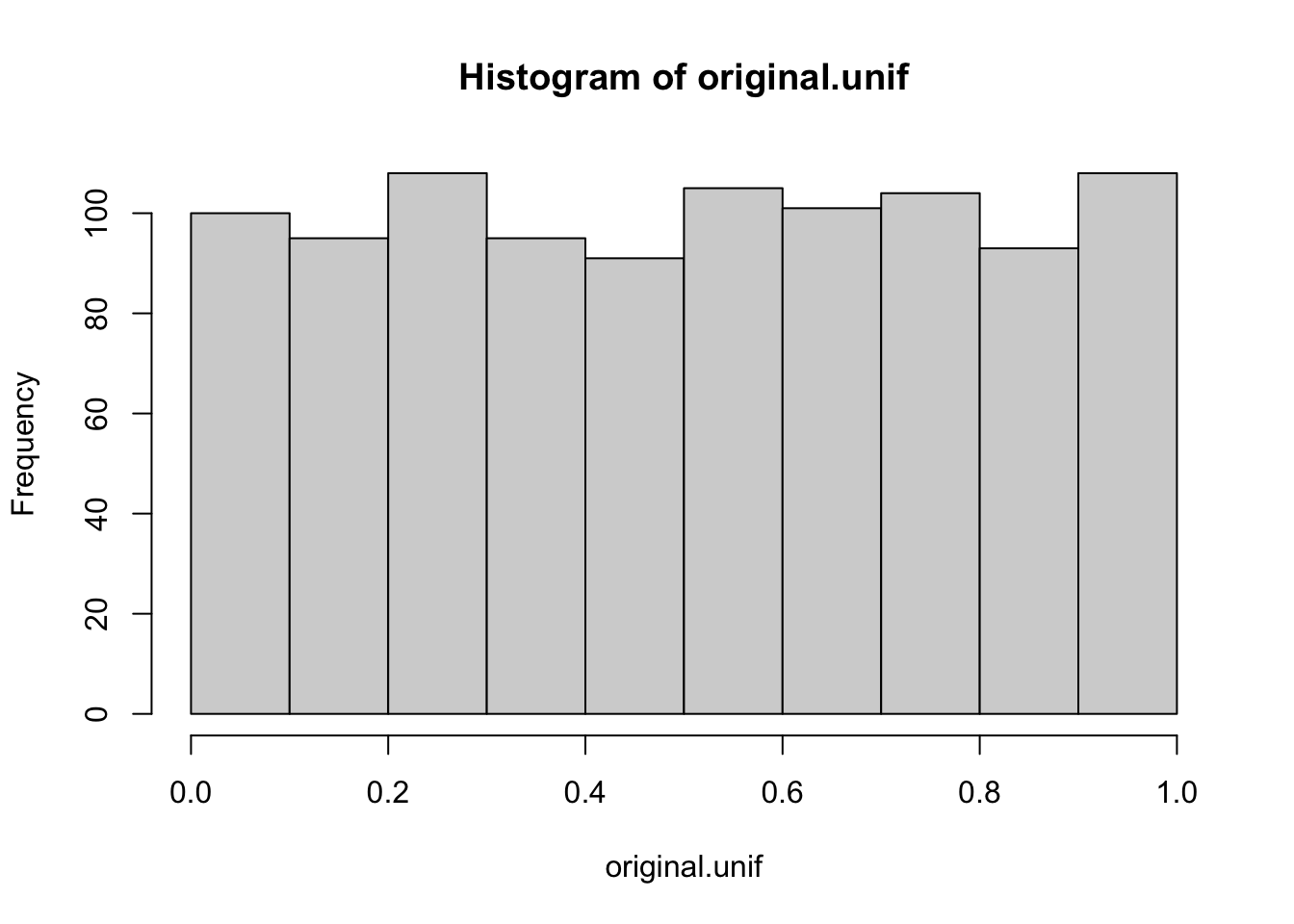 Assume that we know the data are uniformly distributed, but we do not know the upper limit.
We would estimate this limit as the maximum of the data.
Assume that we know the data are uniformly distributed, but we do not know the upper limit.
We would estimate this limit as the maximum of the data.
max(original.unif) %>% round(3)## [1] 0.998If we would now bootstrap this statistic, we would get the following distribution of the statistic:
boot.unif.max <- function(data, ind){
  max(data[ind])
}

booted.unif <- boot(data = original.unif,
                    statistic = boot.unif.max,
                    R = nboot)

hist(booted.unif$t)
abline(v = mean(booted.unif$t), col = "red")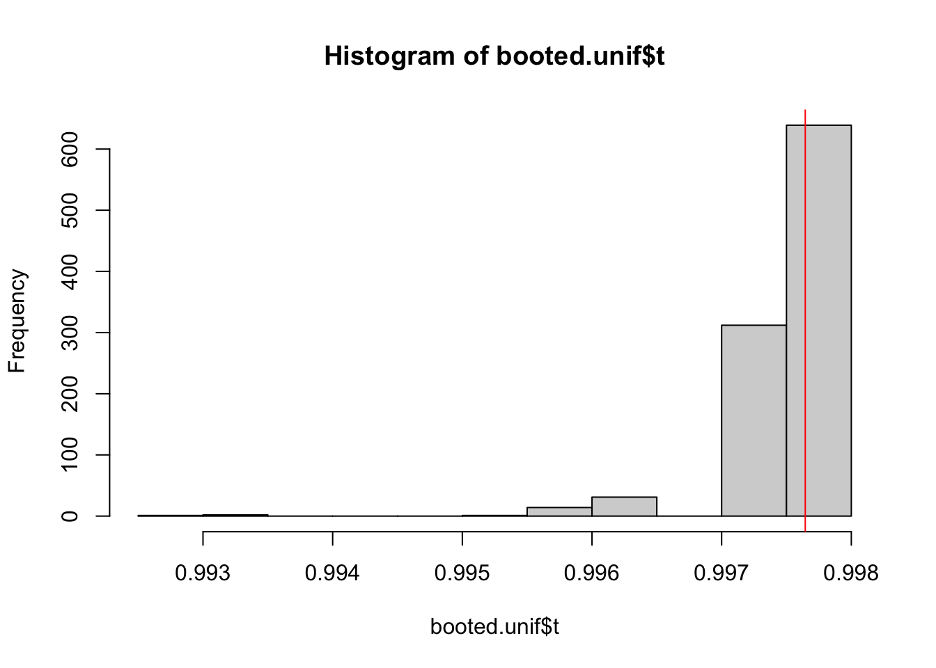
In this case, the bootstrapped estimate is smaller than the original value whenever the maximum value of the original data is not sampled. So all estimates are either as far away of the true parameter, or even more biased (by definition).
Something similar happens if we (for example) try to bootstrap \(R^2\), here because \(R^2\) is a biased estimator. We can see the problem for the case of two independent variables.
I will show the extreme case of two variables with exactly 0 correlation:
original.rsq <- MASS::mvrnorm(n = 100, mu = rep(0, 5),
                     Sigma = diag(x = 1, nrow = 5),
                     empirical = FALSE)
#original.rsq <-data.frame(rnorm(100), rnorm(100))


cor(original.rsq)
## [,1] [,2] [,3] [,4] [,5]
## [1,] 1.000000000 0.0910027 -0.12706723 0.11518181 -0.002021796
## [2,] 0.091002698 1.0000000 -0.04332500 -0.16157754 -0.190770308
## [3,] -0.127067225 -0.0433250 1.00000000 0.01537066 0.096918133
## [4,] 0.115181806 -0.1615775 0.01537066 1.00000000 -0.035044094
## [5,] -0.002021796 -0.1907703 0.09691813 -0.03504409 1.000000000original.rsq <- data.frame("Y" = original.rsq[,1],
"X1" = original.rsq[,2],
"X2" = original.rsq[,3],
"X3" = original.rsq[,4],
"X4" = original.rsq[,5])
orig.rsq.est <- summary(lm(Y ~ X1 + X2 + X3 + X4, data = original.rsq))$r.squaredBecause the variables are empirically uncorrelated, the original \(R^2\) is essentially 0. But if we bootstrap this estimate, the estimate distribution will not be around 0, as \(R^2\) will never be negative, no matter which way the coefficient estimate tilts.
boot.rsq <- function(data, ind){
  data <- data[ind,]
  summary(lm(Y ~ X1 + X2 + X3 + X4, data = data))$r.squared
}

booted.rsq <- boot(data = original.rsq,
                    statistic = boot.rsq,
                    R = nboot)

hist(booted.rsq$t)
abline(v = mean(booted.rsq$t), col = "red")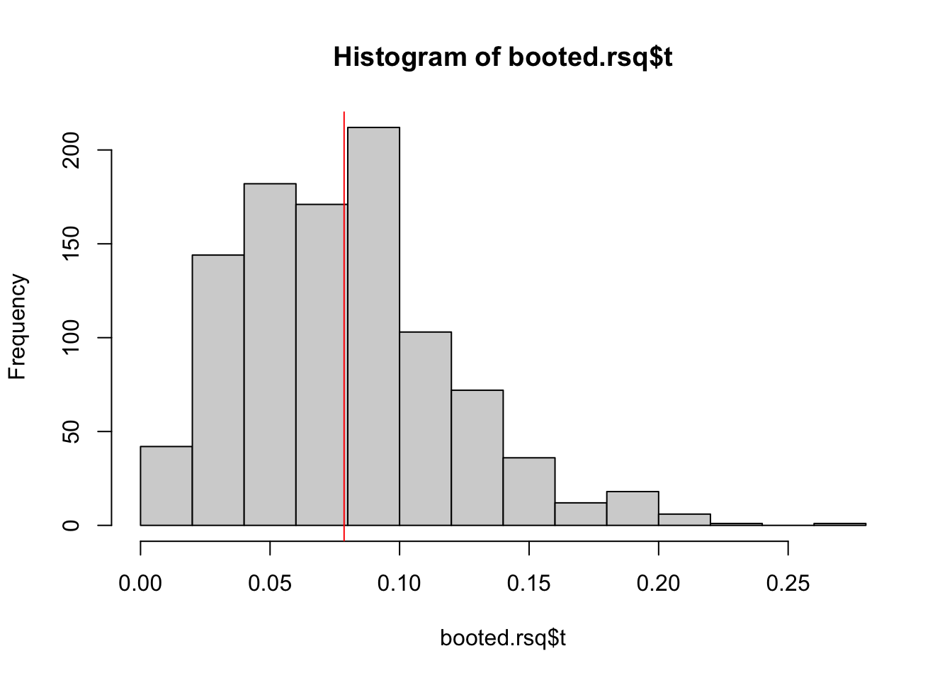
And the percentile CI would not include 0:
boot.ci(booted.rsq, type = "perc")## BOOTSTRAP CONFIDENCE INTERVAL CALCULATIONS
## Based on 1000 bootstrap replicates
##
## CALL :
## boot.ci(boot.out = booted.rsq, type = "perc")
##
## Intervals :
## Level Percentile
## 95% ( 0.0156, 0.1822 )
## Calculations and Intervals on Original Scale