8 Mean Comparisons: T-Tests and ANOVA Models
8.1 T-Tests
8.1.1 One-sample t-test
Sometimes we want to compare a sample mean with a known population mean \((\mu_0)\) or some other fixed comparison value. For example, we would like to know whether the reported support by friends support_friends differs significantly from the midpoint of the 7-point-Likert scale \((\mu_0=4)\).
The required function is t.test(). For the one-sample t-test, we only need the following arguments (incl. default values): alternative = c("two.sided", "less", "greater"), mu = 0, and conf.level = .95.
load(file = "data/adolescents.Rdata")
TTest <- adolescents$support_friends %>%
    t.test(alternative = 'two.sided',
           mu = 4,
           conf.level = .95)
TTest
##
## One Sample t-test
##
## data: .
## t = 33.781, df = 284, p-value < 2.2e-16
## alternative hypothesis: true mean is not equal to 4
## 95 percent confidence interval:
## 5.815396 6.040043
## sample estimates:
## mean of x
##  5.927719
The output of the t.test() function is a list of the object class “htest” (hypothesis test).
typeof(TTest)## [1] "list"attributes(TTest)## $names
## [1] "statistic" "parameter" "p.value" "conf.int" "estimate"
## [6] "null.value" "stderr" "alternative" "method" "data.name"
##
## $class
## [1] "htest"The elements of this list can be selected individually. The (estimated) means can be obtained with:
TTest$estimate## mean of x
## 5.927719The \(p\)-value is returned with:
TTest$p.value## [1] 1.75588e-101Degrees of freedom:
TTest$parameter## df
## 284Confidence Interval:
TTest$conf.int## [1] 5.815396 6.040043
## attr(,"conf.level")
## [1] 0.95The result shows that the sample mean (5.93) is signficantly different from the midpoint of the scale (=4).
By default we obtained a two-sided test for \((H_1:\mu\neq\mu_0)\). One-sided tests are obtained with alternative = "greater" \((H_1:\mu>\mu_0\) or alternative = "less" \((H_1:\mu<\mu_0)\).
One-sample t-test with jmv:
library(jmv)
ttestOneS(
    data = adolescents,
    vars = "support_friends",
    wilcoxon = FALSE,       # if TRUE -> Nonparametric Wilcoxon Rank Sum Test
    testValue = 4,          # a number specifying the value of the null hypothesis (mu0)
    hypothesis = "dt",      # 'dt' (different to - default), 'gt' (greater than),
                            # 'lt' (less than)
    norm = TRUE,            # test for normality of the DV (Shapiro-Wilk test)
    meanDiff = TRUE,        # display estimated mean difference
    effectSize = FALSE,     # Cohen's d
    ci = TRUE,              # confidence interval of the mean difference
    ciWidth = 99,           # CI width default: 95%
    desc = TRUE)            # descriptive statistics
##
## ONE SAMPLE T-TEST
##
## One Sample T-Test
## ────────────────────────────────────────────────────────────────────────────────────────────────────────────────────
## Statistic df p Mean difference Lower Upper
## ────────────────────────────────────────────────────────────────────────────────────────────────────────────────────
## support_friends Student's t 33.78135 284.0000 < .0000001 1.927719 1.779736 2.075702
## ────────────────────────────────────────────────────────────────────────────────────────────────────────────────────
## Note. Hₐ μ ≠ 4
##
##
## Normality Test (Shapiro-Wilk)
## ──────────────────────────────────────────────
## W p
## ──────────────────────────────────────────────
## support_friends 0.8922262 < .0000001
## ──────────────────────────────────────────────
## Note. A low p-value suggests a violation
## of the assumption of normality
##
##
## Descriptives
## ─────────────────────────────────────────────────────────────────────────────
## N Mean Median SD SE
## ─────────────────────────────────────────────────────────────────────────────
## support_friends 285 5.927719 6.000000 0.9633613 0.05706460
## ─────────────────────────────────────────────────────────────────────────────8.1.2 Independent samples t-test
t.test() works also For the independent samples t-test. In this case, the test variable and the factor are specified in the formula notation typical for R: variable ~ factor (\(\rightarrow\) “variable by factor” = “test variable is predicted by factor” = “test the DV mean difference between the two levels of the factor”).
Furthermore, it has to be indicated whether the assumption of equal variances holds in the two groups: for var.equal = FALSE (default), the Welch Two Sample t-test (heteroscedasticity corrected t-test) is applied, for var.equal = TRUE the standard Student’s t-test.
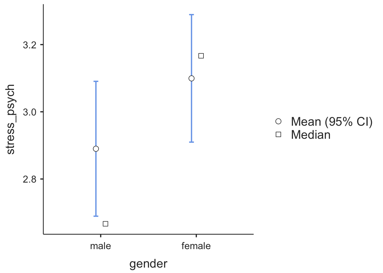
Again, different alternative hypotheses can be specified. For directional hypotheses (one-sided tests), the order of the factor levels has to be considered. For example, if we assume that girls will report a higher level of psychological stress symptoms than boys and the factor gender has as its first level male (as is the case in our dataset since the order of factor levels was defined by the order present in the SPSS data file we imported), the correct alternative hypothesis is \(H_1:\mu_{male} < \mu_{female}\). The required argument is alternative = "less" since formally the mean difference of the two groups is compared to 0, thus in our case \(H_1:\mu_{male}-\mu_{female}<0\).
Let’s assume first that the population variances of stress_psych are equal for boys and girls and carry out the “normal” t-test:
levels(adolescents$gender) # verify order of levels for direction of one-sided hypothesis## [1] "male" "female"t.test(stress_psych ~ gender, alternative = "less",
conf.level = .95,
var.equal = TRUE,
data = adolescents)##
## Two Sample t-test
##
## data: stress_psych by gender
## t = -1.4774, df = 282, p-value = 0.07034
## alternative hypothesis: true difference in means between group male and group female is less than 0
## 95 percent confidence interval:
## -Inf 0.02451332
## sample estimates:
## mean in group male mean in group female
## 2.890000 3.099502To check the assumption of homoscedasticity, we perform the Levene test using the function leveneTest() from the car package. In addition to the test variable and the factor we have to specify whether mean or median should be used for the deviations: for center = mean the (actual) Levene test is performed, for center = median (default) the Brown-Forsythe test, a more robust variant of the Levene test is performed.
library(car)
leveneTest(adolescents$stress_psych, adolescents$gender,
           center = median)
## Levene's Test for Homogeneity of Variance (center = median)
## Df F value Pr(>F)
## group 1 0.5958 0.4408
## 282Since the Levene test is non-significant we can assume homoscedasticity.
Independent samples t-test with jmv
library(jmv)
ttestIS(
  formula = stress_psych ~ gender,
  data = adolescents,
  vars = stress_psych,
  bf = TRUE,                  # Bayes Factor!
  welchs = TRUE,              # Welch's Test
  mann = TRUE,                # Wilcoxon / Mann-Whitney
  hypothesis = "twoGreater",  # 'different' (default),
                              # 'oneGreater' (group 1 greater than group 2)
                              # 'twoGreater' (group 2 greater than group 1)
                              #  Equality of Variances (Levene test)
  qq = TRUE,
  eqv = TRUE,                 # Levene Test
  meanDiff = TRUE,
  effectSize = TRUE,
  desc = TRUE,
  plots = TRUE)
##
## INDEPENDENT SAMPLES T-TEST
##
## Independent Samples T-Test
## ───────────────────────────────────────────────────────────────────────────────────────────────────────────────────────────────────────────────────────────────────────
## Statistic error % df p Mean difference SE difference Effect Size
## ───────────────────────────────────────────────────────────────────────────────────────────────────────────────────────────────────────────────────────────────────────
## stress_psych Student's t -1.477407 282.0000 0.0703412 -0.2095025 0.1418041 Cohen's d -0.1756149
## Bayes factor₁₀ 0.6820815 2.563522e-6
## Welch's t -1.486798 281.9999 0.0690927 -0.2095025 0.1409085 Cohen's d -0.1761724
## Mann-Whitney U 8662.500 0.0222206 -0.3333095 Rank biserial correlation 0.1380597
## ───────────────────────────────────────────────────────────────────────────────────────────────────────────────────────────────────────────────────────────────────────
## Note. Hₐ μ <sub>male</sub> < μ <sub>female</sub>
##
##
## ASSUMPTIONS
##
## Homogeneity of Variances Test (Levene's)
## ──────────────────────────────────────────────────────
## F df df2 p
## ──────────────────────────────────────────────────────
## stress_psych 1.036834 1 282 0.3094318
## ──────────────────────────────────────────────────────
## Note. A low p-value suggests a violation of the
## assumption of equal variances
##
##
## Group Descriptives
## ───────────────────────────────────────────────────────────────────────────────────
## Group N Mean Median SD SE
## ───────────────────────────────────────────────────────────────────────────────────
## stress_psych male 150 2.890000 2.666667 1.254057 0.1023933
## female 134 3.099502 3.166667 1.120575 0.09680296
## ───────────────────────────────────────────────────────────────────────────────────
8.1.3 Paired samples t-test
For this test we can we can again use the base R function t.test().
As an example, we would like to test whether the extent of the support received from parents support_parents differs from the extent of the support received from friends support_friends across the whole sample. This makes sense sine the items underlying support_parents and support_friends are exactly the same, they only differ in the reference given to parents or friends, e.g.:
“My parents (friends) encourage me when I am disappointed or frustrated.”
There are two options: Either we leave the dataset in wide format, where we have support_parents and support_friends as two variables (columns) in the dataset next to each other.
In this case, the data assignment for the t.test () function is not done using the formula notation but by specifying the two variables to be compared. The only difference to the t-test for independent samples is that we specify the option paired = TRUE (default: paired = FALSE), reflecting the dependence of the data in the two samples/variables.
t.test(adolescents$support_parents, adolescents$support_friends,
       alternative = "two.sided",
       conf.level = .95,
       paired = TRUE)
##
## Paired t-test
##
## data: adolescents$support_parents and adolescents$support_friends
## t = -0.73804, df = 283, p-value = 0.4611
## alternative hypothesis: true difference in means is not equal to 0
## 95 percent confidence interval:
## -0.21046776 0.09567902
## sample estimates:
## mean of the differences
## -0.05739437Note that if paired = TRUE would not be specified here, t.test() would assume that the data in the columns support_parents and support_friends be two independent samples!
The second option is to convert the dataset from wide to long, taking into account that parents and friends are actually two levels of a factor, that is the source of the support. The measured variable is support (for both factor levels).
library(tidyverse)
sup_long <- adolescents %>%
    drop_na(support_parents, support_friends) %>%
   dplyr::select(ID, support_parents, support_friends) %>%
    pivot_longer(-ID, names_to = "source", values_to = "support") %>%
    mutate(source = str_replace(source, ".*_", "")) %>%   # remove support_ from
                                                          # source factor levels
    mutate(source = factor(source))                       # define as factor

head(sup_long)
## # A tibble: 6 × 3
## ID source support
## <fct> <fct> <dbl>
## 1 1 parents 6.67
## 2 1 friends 6.67
## 3 2 parents 5.17
## 4 2 friends 4.83
## 5 10 parents 6.83
## 6 10 friends 4sup_long %>%
group_by(source) %>%
summarize(mean = mean(support) %>% round(3),
N = length(support))## # A tibble: 2 × 3
## source mean N
## <fct> <dbl> <int>
## 1 friends 5.93 284
## 2 parents 5.87 284t.test(support ~ source,
alternative = "two.sided",
conf.level = .95,
paired = TRUE,
data = sup_long)##
## Paired t-test
##
## data: support by source
## t = 0.73804, df = 283, p-value = 0.4611
## alternative hypothesis: true difference in means is not equal to 0
## 95 percent confidence interval:
## -0.09567902 0.21046776
## sample estimates:
## mean of the differences
## 0.057394378.2 ANOVA models
8.2.1 One-way analysis of variance
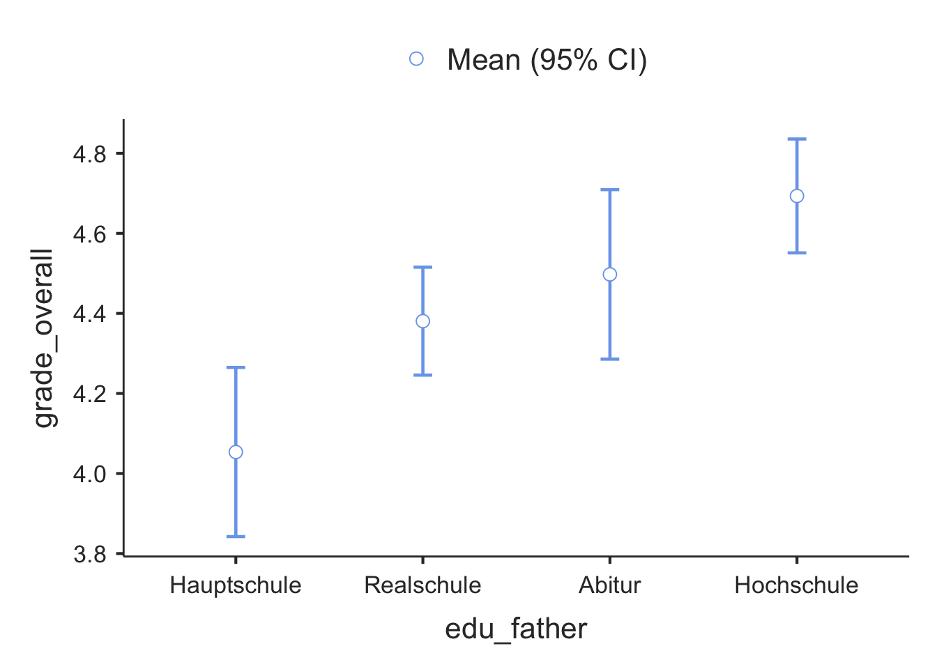
We perform a one-way ANOVA with the grade average grade_overall as the dependent variable and the father’s level of education (edu_father) as a factor (independent variable).
First, we create a data set grades containing only the variables ID,grade_overall, edu_father and gender (for later analysis) and remove all observations with missing values.
grades <- adolescents %>%
   dplyr::select(ID, grade_overall, edu_father, gender) %>%
    drop_na()

grades
## # A tibble: 264 × 4
## ID grade_overall edu_father gender
## <fct> <dbl> <fct> <fct>
## 1 2 4 Abitur male
## 2 10 5 Realschule female
## 3 11 4 Realschule female
## 4 12 5 Hochschule female
## 5 14 4 Realschule male
## 6 15 4 Realschule male
## 7 16 5 Hochschule female
## 8 17 4 Realschule male
## 9 18 4 Abitur male
## 10 19 4 Hauptschule male
## # … with 254 more rowsFirst, let’s look at some descriptive statistics (means and standard deviations) using summarise():
grades %>%
  group_by(edu_father) %>%
  summarise(mean = round(mean(grade_overall, na.rm = TRUE), 2),
            sd = round(sd(grade_overall, na.rm = TRUE), 2),
            N = length(grade_overall))
## # A tibble: 4 × 4
## edu_father mean sd N
## <fct> <dbl> <dbl> <int>
## 1 Hauptschule 4.05 0.67 41
## 2 Realschule 4.38 0.65 93
## 3 Abitur 4.5 0.65 39
## 4 Hochschule 4.69 0.68 91Descriptively, higher educational levels of the father are related to a higher overall grade average of students. Also, the standard deviations of the DV seem to be similar across groups. leveneTest() is used to test the assumption of homogeneity of variances.
library(car)
leveneTest(grades$grade_overall, grades$edu_father,
           center = median)
## Levene's Test for Homogeneity of Variance (center = median)
## Df F value Pr(>F)
## group 3 0.4906 0.6891
## 260The non-significance of the Levene test allows to maintain the assumption of homoscedasticity.
Now we can compute the ANOVA using the aov() function, save the output in a results object and then use the summary() function to access the output. aov() is a wrapper function for the more general lm() function (linear model, see next chapter) designed to extract the relevant information for an ANOVA-type of analysis (which is based on a general linear model or GLM).
The TukeyHSD function can be used to get all pairwise comparisons (adjusted confidence intervals and Tukey \(p\)-values).
anova1 <- aov(grade_overall ~ edu_father, data = grades)
summary(anova1)
## Df Sum Sq Mean Sq F value Pr(>F)
## edu_father 3 12.36 4.120 9.272 7.58e-06 ***
## Residuals 260 115.53 0.444
## ---
## Signif. codes: 0 '***' 0.001 '**' 0.01 '*' 0.05 '.' 0.1 ' ' 1TukeyHSD(anova1, ordered = TRUE)## Tukey multiple comparisons of means
## 95% family-wise confidence level
## factor levels have been ordered
##
## Fit: aov(formula = grade_overall ~ edu_father, data = grades)
##
## $edu_father
## diff lwr upr p adj
## Realschule-Hauptschule 0.3269866 0.003864173 0.6501091 0.0461134
## Abitur-Hauptschule 0.4437774 0.058237843 0.8293169 0.0167437
## Hochschule-Hauptschule 0.6397481 0.315540988 0.9639551 0.0000039
## Abitur-Realschule 0.1167907 -0.212031612 0.4456131 0.7950495
## Hochschule-Realschule 0.3127614 0.058608643 0.5669142 0.0088548
## Hochschule-Abitur 0.1959707 -0.133917530 0.5258589 0.4174570Beside the TukeyHSD() function there is another way to obtain post-hoc pairwise comparisons: pairwise.t.test()
Among others, the methods p.adjust.method = c("bonferroni", "holm") are available. The pairwise.t.test() function works independently of the ANOVA procedure (it performs pairwise adjusted t-tests without an overall test).
pairwise.t.test(grades$grade_overall, grades$edu_father,
                p.adjust.method = "bonferroni")
##
## Pairwise comparisons using t tests with pooled SD
##
## data: grades$grade_overall and grades$edu_father
##
## Hauptschule Realschule Abitur
## Realschule 0.0564 - -
## Abitur 0.0192 1.0000 -
## Hochschule 3.9e-06 0.0098 0.7544
##
## P value adjustment method: bonferronipairwise.t.test(grades$grade_overall, grades$edu_father,
p.adjust.method = "holm")##
## Pairwise comparisons using t tests with pooled SD
##
## data: grades$grade_overall and grades$edu_father
##
## Hauptschule Realschule Abitur
## Realschule 0.0282 - -
## Abitur 0.0128 0.3593 -
## Hochschule 3.9e-06 0.0082 0.2515
##
## P value adjustment method: holmOne-way ANOVA in jmv: Like SPSS, jmv provides different procedures (and syntax) for one-way and factorial ANOVA.
anovaOneW(
    formula = grade_overall ~ edu_father,
    data = adolescents,
    fishers = TRUE,
    desc = TRUE,
    descPlot = TRUE,
    qq = TRUE,
    eqv = TRUE,
    phMethod = "tukey",
    phTest = TRUE)
##
## ONE-WAY ANOVA
##
## One-Way ANOVA
## ─────────────────────────────────────────────────────────────────────────
## F df1 df2 p
## ─────────────────────────────────────────────────────────────────────────
## grade_overall Welch's 8.951002 3 108.3205 0.0000238
## Fisher's 9.272342 3 260 0.0000076
## ─────────────────────────────────────────────────────────────────────────
##
##
## Group Descriptives
## ─────────────────────────────────────────────────────────────────────────────
## edu_father N Mean SD SE
## ─────────────────────────────────────────────────────────────────────────────
## grade_overall Hauptschule 41 4.053659 0.6693645 0.10453717
## Realschule 93 4.380645 0.6546254 0.06788149
## Abitur 39 4.497436 0.6531249 0.10458369
## Hochschule 91 4.693407 0.6829352 0.07159106
## ─────────────────────────────────────────────────────────────────────────────
##
##
## ASSUMPTION CHECKS
##
## Homogeneity of Variances Test (Levene's)
## ─────────────────────────────────────────────────────────
## F df1 df2 p
## ─────────────────────────────────────────────────────────
## grade_overall 0.6032603 3 260 0.6134189
## ─────────────────────────────────────────────────────────
##
##
## POST HOC TESTS
##
## Tukey Post-Hoc Test – grade_overall
## ───────────────────────────────────────────────────────────────────────────────────────────
## Hauptschule Realschule Abitur Hochschule
## ───────────────────────────────────────────────────────────────────────────────────────────
## Hauptschule Mean difference — -0.3269866 -0.4437774 -0.6397481
## t-value — -2.616645 -2.9763104 -5.102329
## df — 260.0000 260.0000 260.0000
## p-value — 0.0461134 0.0167437 0.0000039
##
## Realschule Mean difference — -0.1167907 -0.3127614
## t-value — -0.9183940 -3.182001
## df — 260.0000 260.0000
## p-value — 0.7950495 0.0088548
##
## Abitur Mean difference — -0.1959707
## t-value — -1.536053
## df — 260.0000
## p-value — 0.4174570
##
## Hochschule Mean difference —
## t-value —
## df —
## p-value —
## ───────────────────────────────────────────────────────────────────────────────────────────
8.2.2 (One-way) repeated measures ANOVA
Let’s look at the fictitious small sample study “Honeymoon or Hangover” (from the book by [Budischewski & Günther, 2020] (https://www.beltz.de/produkt_detailansicht/43909-aufgabensammlung-statistik.html). In this study, \(n = 10\) employees from two companies (\(n = 5\) each) were interviewed at the beginning of their employment (start) as well as at two further measurement points (3_months, 6_months) regarding their job satisfaction (satisfaction). The hypothesis was that employees are very satisfied at the beginning, as they enthusiastically approach the new task (“honeymoon”), then due to the heavy workload at a new entry a phase of lesser satisfaction follows (“hangover”) before satisfaction levels off again (here after six months). In general, we ask about the differences in the mean values of job satisfaction over time. We start with only one company (company 1).
honeymoon <- tibble(ID = factor(rep(1:10, each = 3)),
                    company = factor(rep(1:2, each = 15)),
                    time = factor(rep(c("start", "3_months", "6_months"), times = 10),
                                  levels = c("start", "3_months", "6_months")),
                    satisfaction = c(9, 4, 5, 9, 4, 8, 9, 7, 14, 10, 9, 5, 8, 1,
                    3, 10, 10, 10, 9, 11, 10, 10, 11, 12, 12, 13, 14, 9, 9, 9))
Let’s get the means of the DV:
honeymoon %>%
    group_by(company, time) %>%
    summarise(satisfaction = mean(satisfaction))
## `summarise()` has grouped output by 'company'. You can override using the `.groups` argument.## # A tibble: 6 × 3
## # Groups: company [2]
## company time satisfaction
## <fct> <fct> <dbl>
## 1 1 start 9
## 2 1 3_months 5
## 3 1 6_months 7
## 4 2 start 10
## 5 2 3_months 10.8
## 6 2 6_months 11First, we only want to examine the development of job satisfaction in the first company:
# select company 1
honeymoon_1 <- honeymoon %>%
    filter(company == 1)
First, let’s use the classic aov() method again:
rm_anova <- aov(satisfaction ~ time + Error(ID/time), data = honeymoon_1)

summary(rm_anova)
##
## Error: ID
## Df Sum Sq Mean Sq F value Pr(>F)
## Residuals 4 60 15
##
## Error: ID:time
## Df Sum Sq Mean Sq F value Pr(>F)
## time 2 40 20.00 2.963 0.109
## Residuals 8 54 6.75The package ezANOVA() provides more functionality for repeated measures ANOVAs, including sphericity tests and corrections:
install.packages("ez")
library(ez)
ezANOVA(honeymoon_1, dv = satisfaction,
        wid = ID, within = time,
        detailed = TRUE)
## $ANOVA
## Effect DFn DFd SSn SSd F p p<.05 ges
## 1 (Intercept) 1 4 735 60 49.000000 0.00219213 * 0.8657244
## 2 time 2 8 40 54 2.962963 0.10890896 0.2597403
##
## $`Mauchly's Test for Sphericity`
## Effect W p p<.05
## 2 time 0.6872428 0.569725
##
## $`Sphericity Corrections`
## Effect GGe p[GG] p[GG]<.05 HFe p[HF] p[HF]<.05
## 2 time 0.7617555 0.1308327 1.134177 0.108909Since the Mauchly test is not significant, we can assume a spherical variance-covariance matrix (sphericity assumption). However, because of the low power of the Mauchly test in this small sample study we could still apply the corrections according to Greenhouse Geisser-\(\epsilon\) (GGe) or Huynh-Feldt-$$ (HFe).
The effect of the factor time is not significant, independent of whether sphericity corrections p[GG] and p[HF] are being used or not. Our very small sample of n = 5 is associated with a very low statistical power, though.
Post-hoc tests can be obtained using the pairwise.t.test() from stats, where we have to specify paired = TRUE. Here we use both the uncorrected pairwise comparisons (p.adjust.method = "none") and the Bonferroni-Holm corrected comparisons (p.adjust.method = "holm"). This is done for demonstration purposes even though the overall effect was non-significant.
pairwise.t.test(honeymoon_1$satisfaction,
                honeymoon_1$time,
                p.adjust.method = "none",
                paired = TRUE)
##
## Pairwise comparisons using paired t tests
##
## data: honeymoon_1$satisfaction and honeymoon_1$time
##
## start 3_months
## 3_months 0.022 -
## 6_months 0.351 0.333
##
## P value adjustment method: nonepairwise.t.test(honeymoon_1$satisfaction,
honeymoon_1$time,
p.adjust.method = "holm",
paired = TRUE)##
## Pairwise comparisons using paired t tests
##
## data: honeymoon_1$satisfaction and honeymoon_1$time
##
## start 3_months
## 3_months 0.065 -
## 6_months 0.665 0.665
##
## P value adjustment method: holmWe can do the RM ANOVA also with jmv. In jmv we need a wide dataset since part of the philosophy of jmv and jamovi is to provide similar functionality to former SPSS users.
Let’s apply a long-to-wide transformation to honeymooon_1:
honeymoon_1_wide <- honeymoon_1 %>%
  pivot_wider(names_from = time, values_from = satisfaction)

honeymoon_1_wide
## # A tibble: 5 × 5
## ID company start `3_months` `6_months`
## <fct> <fct> <dbl> <dbl> <dbl>
## 1 1 1 9 4 5
## 2 2 1 9 4 8
## 3 3 1 9 7 14
## 4 4 1 10 9 5
## 5 5 1 8 1 3The syntax of the jmv::anovaRM() function is quite complicated (because of the untidy wide dataset):
anovaRM(
    data = honeymoon_1_wide,
    rm = list(                   # Definition of RM factor / factor levels
        list(
            label = "Time",
            levels = c("Start", "3_Months", "6_Months"))),
    rmCells = list(              # Assignment of the DV (measure)
        list(                    # to the cells (factor levels)
            measure = "start",
            cell = "Start"),
        list(
            measure = "3_months",
            cell = "3_Months"),
        list(
            measure = "6_months",
            cell = "6_Months")),
    rmTerms = list(              # Calling those RM model terms that should
        "Time"),        # be used in the current model
    effectSize = c("eta", "omega"),
    spherTests = TRUE,
    spherCorr = c("none", "GG", "HF"))
##
## REPEATED MEASURES ANOVA
##
## Within Subjects Effects
## ─────────────────────────────────────────────────────────────────────────────────────────────────────────────────────────────────────
## Sphericity Correction Sum of Squares df Mean Square F p η² ω²
## ─────────────────────────────────────────────────────────────────────────────────────────────────────────────────────────────────────
## Time None 40.00000 2 20.000000 2.962963 0.1089090 0.2597403 0.1648523
## Greenhouse-Geisser 40.00000 1.523511 26.255144 2.962963 0.1308327 0.2597403 0.1648523
## Huynh-Feldt 40.00000 2.000000 20.000000 2.962963 0.1089090 0.2597403 0.1648523
##
## Residual None 54.00000 8 6.750000
## Greenhouse-Geisser 54.00000 6.094044 8.861111
## Huynh-Feldt 54.00000 8.000000 6.750000
## ─────────────────────────────────────────────────────────────────────────────────────────────────────────────────────────────────────
## Note. Type 3 Sums of Squares
##
##
## Between Subjects Effects
## ───────────────────────────────────────────────────────────────────────────────────────────────
## Sum of Squares df Mean Square F p η² ω²
## ───────────────────────────────────────────────────────────────────────────────────────────────
## Residual 60.00000 4 15.00000
## ───────────────────────────────────────────────────────────────────────────────────────────────
## Note. Type 3 Sums of Squares
##
##
## ASSUMPTIONS
##
## Tests of Sphericity
## ─────────────────────────────────────────────────────────────────────────────
## Mauchly's W p Greenhouse-Geisser ε Huynh-Feldt ε
## ─────────────────────────────────────────────────────────────────────────────
## Time 0.6872428 0.5697250 0.7617555 1.000000
## ─────────────────────────────────────────────────────────────────────────────# postHoc = "Time",
# postHocCorr = "holm")8.2.3 Factorial ANOVA
2-factors between design
We would like to analyse the joint effect of two factors on adolescents’ grade average: A) educational level of the father (edu_father) and B) gender (gender) .
Again, let’s first look at descriptive statistics using summarise():
 grades %>%
    group_by(edu_father) %>%
    summarise(mean = round(mean(grade_overall, na.rm = TRUE), 2),
             sd = round(sd(grade_overall, na.rm = TRUE), 3),
              var = round(var(grade_overall, na.rm = TRUE), 3),
              N = length(grade_overall))
## # A tibble: 4 × 5
## edu_father mean sd var N
## <fct> <dbl> <dbl> <dbl> <int>
## 1 Hauptschule 4.05 0.669 0.448 41
## 2 Realschule 4.38 0.655 0.429 93
## 3 Abitur 4.5 0.653 0.427 39
## 4 Hochschule 4.69 0.683 0.466 91 grades %>%
group_by(gender) %>%
summarise(mean = round(mean(grade_overall, na.rm = TRUE), 2),
sd = round(sd(grade_overall, na.rm = TRUE), 3),
var = round(var(grade_overall, na.rm = TRUE), 3),
N = length(grade_overall))## # A tibble: 2 × 5
## gender mean sd var N
## <fct> <dbl> <dbl> <dbl> <int>
## 1 male 4.29 0.723 0.522 145
## 2 female 4.65 0.612 0.375 119Then we carry out the Levene test to check the homoscadasticity assumption:
library(car)
leveneTest(grades$grade_overall ~ grades$edu_father*grades$gender,
           center = median)
## Levene's Test for Homogeneity of Variance (center = median)
## Df F value Pr(>F)
## group 7 1.1221 0.3495
## 256First, we perform the two-factorial analysis of variance using aov():
anova2 <- aov(grade_overall ~ edu_father*gender, data = grades)
Anova(anova2, type = 3)
## Anova Table (Type III tests)
##
## Response: grade_overall
## Sum Sq Df F value Pr(>F)
## (Intercept) 328.41 1 799.1587 < 2.2e-16 ***
## edu_father 9.90 3 8.0335 3.891e-05 ***
## gender 1.71 1 4.1714 0.04214 *
## edu_father:gender 0.85 3 0.6875 0.56041
## Residuals 105.20 256
## ---
## Signif. codes: 0 '***' 0.001 '**' 0.01 '*' 0.05 '.' 0.1 ' ' 1A full-factorial model including all main effects and interactions is specified by combining the factors using the multiplication sign on the right-hand side of the formula: factor_A*factor_B. This is equivalent to factorA + factorB + factorA:factorB.
For factorial ANOVAS it is essential to request the summary of the ANOVA object using Anova() from the car package. Only this way Type II or Type III sums of squares (type = 2 ortype = 3) can be obtained. summary() only returns Type I sums of squares (no further option).
The most common method (and the one known from SPSS) is Type III sums of squares where all levels of effect terms are partialled for each other (in terms of cell frequencies in unbalanced designs). The default for Anova() is type = 2 since some important developers for statistical analyses in R prefer Type II sums of squares that return marginal sums of squares for lower order effects (not partialled for higher order effects; here: main effects independent of the interaction effect). Finally, Type I sums of squares return a sequential partialization of all effects (including those of the same order; here: only the main effect that enters the model second is partialled for the one entered first, but not the other way round as in Type II).
Let’s look at the differences:
anova3 <- aov(grade_overall ~ edu_father*gender, data = grades)
Anova(anova3, type = 2)
## Anova Table (Type II tests)
##
## Response: grade_overall
## Sum Sq Df F value Pr(>F)
## edu_father 13.421 3 10.8863 9.380e-07 ***
## gender 9.484 1 23.0781 2.651e-06 ***
## edu_father:gender 0.848 3 0.6875 0.5604
## Residuals 105.202 256
## ---
## Signif. codes: 0 '***' 0.001 '**' 0.01 '*' 0.05 '.' 0.1 ' ' 1# anova3 has the same main effects sum of squares as the following model:
anova4 <- aov(grade_overall ~ edu_father + gender, data = grades)
Anova(anova4, type = 2)## Anova Table (Type II tests)
##
## Response: grade_overall
## Sum Sq Df F value Pr(>F)
## edu_father 13.421 3 10.926 8.827e-07 ***
## gender 9.484 1 23.162 2.533e-06 ***
## Residuals 106.049 259
## ---
## Signif. codes: 0 '***' 0.001 '**' 0.01 '*' 0.05 '.' 0.1 ' ' 1# Sequential partialling (Type I) A:
anova5 <- aov(grade_overall ~ edu_father*gender, data = grades)
summary(anova5)## Df Sum Sq Mean Sq F value Pr(>F)
## edu_father 3 12.36 4.120 10.026 2.86e-06 ***
## gender 1 9.48 9.484 23.078 2.65e-06 ***
## edu_father:gender 3 0.85 0.283 0.687 0.56
## Residuals 256 105.20 0.411
## ---
## Signif. codes: 0 '***' 0.001 '**' 0.01 '*' 0.05 '.' 0.1 ' ' 1# Sequential partialling (Type I) B:
anova6 <- aov(grade_overall ~ gender*edu_father, data = grades)
summary(anova6)## Df Sum Sq Mean Sq F value Pr(>F)
## gender 1 8.42 8.424 20.498 9.15e-06 ***
## edu_father 3 13.42 4.474 10.886 9.38e-07 ***
## gender:edu_father 3 0.85 0.283 0.687 0.56
## Residuals 256 105.20 0.411
## ---
## Signif. codes: 0 '***' 0.001 '**' 0.01 '*' 0.05 '.' 0.1 ' ' 1Factorial ANOVA with jmv includes options for contrast analysis and post-hoc comparisons.
ANOVA(
  formula = grade_overall ~ edu_father + gender + edu_father:gender,
  data = adolescents,
  effectSize = c("eta", "partEta", "omega"),
  modelTest = TRUE,
  ss = "3",
  homo = TRUE,
  contrasts = list(
    list(
      var="edu_father",
      type="helmert"),
    list(
      var="gender",
      type="none")))
##
## ANOVA
##
## ANOVA - grade_overall
## ─────────────────────────────────────────────────────────────────────────────────────────────────────────────────────────────────
## Sum of Squares df Mean Square F p η² η²p ω²
## ─────────────────────────────────────────────────────────────────────────────────────────────────────────────────────────────────
## Overall model 20.8801758 7 2.9828823 7.8884837 < .0000001
## edu_father 12.7168152 3 4.2389384 10.3151356 0.0000020 0.1008617 0.1078442 0.0907877
## gender 7.3157984 1 7.3157984 17.8024414 0.0000340 0.0580243 0.0650193 0.0545870
## edu_father:gender 0.8475622 3 0.2825207 0.6874928 0.5604118 0.0067223 0.0079922 -0.0030458
## Residuals 105.2015481 256 0.4109435
## ─────────────────────────────────────────────────────────────────────────────────────────────────────────────────────────────────
##
##
## ASSUMPTION CHECKS
##
## Homogeneity of Variances Test (Levene's)
## ────────────────────────────────────────
## F df1 df2 p
## ────────────────────────────────────────
## 1.539667 7 256 0.1541807
## ────────────────────────────────────────
##
##
## CONTRASTS
##
## Contrasts - edu_father
## ──────────────────────────────────────────────────────────────────────────────────────────────────────
## Estimate SE t p
## ──────────────────────────────────────────────────────────────────────────────────────────────────────
## Hauptschule - Realschule, Abitur, Hochschule -0.4699210 0.11075244 -4.242985 0.0000309
## Realschule - Abitur, Hochschule -0.2243302 0.09079138 -2.470832 0.0141318
## Abitur - Hochschule -0.2132239 0.12360783 -1.725003 0.0857337
## ──────────────────────────────────────────────────────────────────────────────────────────────────────# postHoc = ~ edu_father,
# postHocCorr = c("none", "bonf", "holm"))Mixed (within-between) design ANOVA
We now want to compare the development of job satisfaction across the two companies.
honeymoon %>%
    group_by(company, time) %>%
    summarise(satisfaction = mean(satisfaction))
## `summarise()` has grouped output by 'company'. You can override using the `.groups` argument.## # A tibble: 6 × 3
## # Groups: company [2]
## company time satisfaction
## <fct> <fct> <dbl>
## 1 1 start 9
## 2 1 3_months 5
## 3 1 6_months 7
## 4 2 start 10
## 5 2 3_months 10.8
## 6 2 6_months 11With aov() the mixed-design ANOVA is obtained by:
mixed_anova <- aov(satisfaction ~ company*time + Error(ID/time), data = honeymoon)

summary(mixed_anova)
##
## Error: ID
## Df Sum Sq Mean Sq F value Pr(>F)
## company 1 97.2 97.20 8.877 0.0176 *
## Residuals 8 87.6 10.95
## ---
## Signif. codes: 0 '***' 0.001 '**' 0.01 '*' 0.05 '.' 0.1 ' ' 1
##
## Error: ID:time
## Df Sum Sq Mean Sq F value Pr(>F)
## time 2 13.4 6.700 1.874 0.1857
## company:time 2 29.4 14.700 4.112 0.0362 *
## Residuals 16 57.2 3.575
## ---
## Signif. codes: 0 '***' 0.001 '**' 0.01 '*' 0.05 '.' 0.1 ' ' 1There are aov() formula notations for more ad advanced ANOVA designs (http://www.cookbook-r.com/Statistical_analysis/ANOVA/):
Two within factors
ww_anova <- aov(y ~ RM1*RM2 + Error(subject/(w1*w2)), data = data)
One between factor and two within factors
bww_anova <- aov(y ~ b1*w1*w2 + Error(subject/(w1*w2)) + b1, data = data)
Two between factors and one within factor
bbw_anova <- aov(y ~ b1*b2*w1 + Error(subject/(w1)) + b1*b2, data = data)
With ezANOVA() the mixed-design ANOVA is obtained by defining the variable time as within-factor and company as between-factor:
library(ez)
ezANOVA(honeymoon, dv = satisfaction,
        wid = ID, within = time,
        between = company, detailed = TRUE)
## $ANOVA
## Effect DFn DFd SSn SSd F p p<.05 ges
## 1 (Intercept) 1 8 2323.2 87.6 212.164384 4.837731e-07 * 0.94132901
## 2 company 1 8 97.2 87.6 8.876712 1.761704e-02 * 0.40165289
## 3 time 2 16 13.4 57.2 1.874126 1.856652e-01 0.08470291
## 4 company:time 2 16 29.4 57.2 4.111888 3.622639e-02 * 0.16877153
##
## $`Mauchly's Test for Sphericity`
## Effect W p p<.05
## 3 time 0.7122598 0.3049541
## 4 company:time 0.7122598 0.3049541
##
## $`Sphericity Corrections`
## Effect GGe p[GG] p[GG]<.05 HFe p[HF] p[HF]<.05
## 3 time 0.7765541 0.19689735 0.9289728 0.18928790
## 4 company:time 0.7765541 0.05071043 0.9289728 0.04029652 *To do this in jmv we need the wide data set again now, including both companies:
honeymoon_wide <- honeymoon %>%
  pivot_wider(names_from = time, values_from = satisfaction)

honeymoon_wide
## # A tibble: 10 × 5
## ID company start `3_months` `6_months`
## <fct> <fct> <dbl> <dbl> <dbl>
## 1 1 1 9 4 5
## 2 2 1 9 4 8
## 3 3 1 9 7 14
## 4 4 1 10 9 5
## 5 5 1 8 1 3
## 6 6 2 10 10 10
## 7 7 2 9 11 10
## 8 8 2 10 11 12
## 9 9 2 12 13 14
## 10 10 2 9 9 9We get the mixed-design ANOVA by adding the arguments bs = 'company' (definition of the between subjects factor) and bsTerms = "company" to the previous code for the RM ANOVA. The latter argument indicates which of the factors listed under bs should be used in the model. The interaction effect between the bs factor and the rm factor is included automatically.
anovaRM(
    data = honeymoon_wide,
    rm = list(                   # Definition of RM factor / factor levels
        list(
            label = "Time",
            levels = c("Start", "3_Months", "6_Months"))),
    rmCells = list(              # Assignment of the DV (measure)
        list(                    # to the cells (factor levels)
            measure = "start",
            cell = "Start"),
        list(
            measure = "3_months",
            cell = "3_Months"),
        list(
            measure = "6_months",
            cell = "6_Months")),
    rmTerms = list(              # Calling those RM model terms that should
        "Time"),                 # be used in the current model
        bs = "company",          # Definition of between factor
    bsTerms = list(              # Calling those "between" model terms that should
        "company"),              # be used in the current model
    effectSize = c("eta", "omega"),
    spherTests = TRUE,
    spherCorr = c("none", "GG", "HF"))
##
## REPEATED MEASURES ANOVA
##
## Within Subjects Effects
## ──────────────────────────────────────────────────────────────────────────────────────────────────────────────────────────────────────────
## Sphericity Correction Sum of Squares df Mean Square F p η² ω²
## ──────────────────────────────────────────────────────────────────────────────────────────────────────────────────────────────────────────
## Time None 13.40000 2 6.700000 1.874126 0.1856652 0.0470506 0.0216732
## Greenhouse-Geisser 13.40000 1.553108 8.627860 1.874126 0.1968973 0.0470506 0.0216732
## Huynh-Feldt 13.40000 1.857946 7.212267 1.874126 0.1892879 0.0470506 0.0216732
##
## Time:company None 29.40000 2 14.700000 4.111888 0.0362264 0.1032303 0.0771565
## Greenhouse-Geisser 29.40000 1.553108 18.929781 4.111888 0.0507104 0.1032303 0.0771565
## Huynh-Feldt 29.40000 1.857946 15.823929 4.111888 0.0402965 0.1032303 0.0771565
##
## Residual None 57.20000 16 3.575000
## Greenhouse-Geisser 57.20000 12.424866 4.603671
## Huynh-Feldt 57.20000 14.863565 3.848336
## ──────────────────────────────────────────────────────────────────────────────────────────────────────────────────────────────────────────
## Note. Type 3 Sums of Squares
##
##
## Between Subjects Effects
## ──────────────────────────────────────────────────────────────────────────────────────────────────────
## Sum of Squares df Mean Square F p η² ω²
## ──────────────────────────────────────────────────────────────────────────────────────────────────────
## company 97.20000 1 97.20000 8.876712 0.0176170 0.3412921 0.2916314
## Residual 87.60000 8 10.95000
## ──────────────────────────────────────────────────────────────────────────────────────────────────────
## Note. Type 3 Sums of Squares
##
##
## ASSUMPTIONS
##
## Tests of Sphericity
## ─────────────────────────────────────────────────────────────────────────────
## Mauchly's W p Greenhouse-Geisser ε Huynh-Feldt ε
## ─────────────────────────────────────────────────────────────────────────────
## Time 0.7122598 0.3049541 0.7765541 0.9289728
## ─────────────────────────────────────────────────────────────────────────────When we later look at multilevel or mixed models, we will see that repeated measures ANOVA designs can also be analyzed in the framework of mixed models, and thus with less strict assumptions regarding the covariance structure.