11 Data simulation
pacman::p_load(tidyverse, lme4, simr)11.1 Basics
Most common distributions are implemented in base R.
For a good general overview see this chapter of another R course.
Each distribution has implemented also a quasi-random data generating function starting with r, e.g. rnorm() for normally distributed numbers, or runif() for random uniform numbers.
We can specify parameters for the number generators to generate data according to our prerequisites.
The sample() function is also a very usefull tool.
If we chose the setting replace = TRUE in that function, and leave the default prob setting, we sample according to a discrete uniform distribution over all entries in our sampling vector.
We can, for example, randomly sample 50 values from a normal distribution with \(\mu = 2\) and the standard deviation \(\sigma = 2\). But first, we make the example reproducible by setting a seed:
set.seed(1413)

rnorm(n = 50, mean =  2, sd = 2) %>%
  round(4) %>%
  print() %>% # print out rounded values
  density() %>% # smooth density estimation
  plot() %>% # plot density
  abline(v = 2, col = "red") # add vertical line of true mean
## [1] 2.4067 1.4031 2.9782 0.2701 -1.2127 0.1227 2.6192 4.0750 2.8920
## [10] 6.6612 4.6134 2.0064 0.6730 1.3692 0.1816 2.4681 3.1938 4.2389
## [19] 4.7378 1.4919 3.2757 2.0376 3.3145 3.1323 0.1044 0.6688 -1.9733
## [28] 0.4641 0.8027 -2.6118 1.0727 3.8566 2.5002 0.8582 0.0440 3.8491
## [37] 6.0439 5.5044 1.1016 4.1413 1.3772 5.4016 3.7061 1.2309 -0.1826
## [46] 2.4296 5.6817 1.6379 0.1860 -0.5932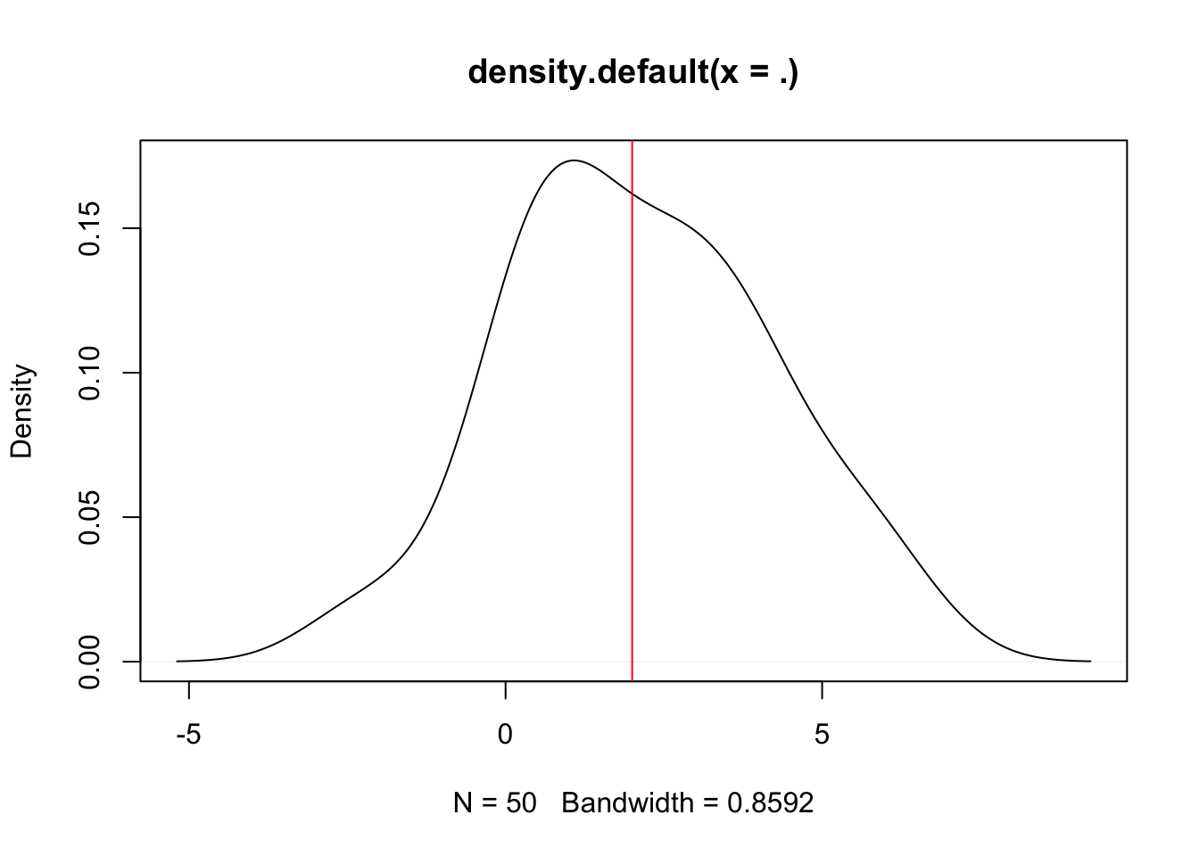
Or we can simulate 10 coin tosses with various functions.
# easiest probably with the sample function:
samp <- sample(c("heads", "tails"), 10, replace = TRUE)

# rbinom
rbino <- rbinom(n = 10, size = 1, prob = .5)

# runif
runi <- runif(n = 10, min = 0, max = 1)
ifelse(runi < 0.5, "heads", "tails")
## [1] "heads" "heads" "heads" "heads" "tails" "heads" "tails" "heads" "tails"
## [10] "tails"11.2 Under H0 (Simulate test statistic)
The idea here is to simulate a test statistic under \(H_0\), whatever \(H_0\) may be. If we can sample under \(H_0\) we can also compare an empirical observation to the distribution under \(H_0\). We can then judge how likely the observed data would be, given that \(H_0\) were true.
Idea of example taken from the Computational Statistics lecture by Marloes Maathuis.
Panini: 1 box contains 100 packs with each 5 stickers. 678 stickers in total for UEFA 2020.
Now we bought half a box, and got only 23 duplicates.
But how many duplicated cards would we expect if stickers are all as common, and independently distributed (this is our \(H_0\))? How likely are 23 duplicates in 250 cards given our \(H_0\)?
set.seed(315)
n.sim <- 1e5 # number of simulations we want to conduct
half.box <- 50*5 # how many stickers in half a box
# n.packs <- 50 # how many packs in half a box
# cards.pack <- 5 # how many cards in a pack
n.cards <- 678 # how many different cards are there?
emp.dupl <- 23 # observed number of duplicated cards in half a box.

# lets simulate one draw:
sample.cards <- sample(1:n.cards, size = half.box, replace = TRUE)
sample.stat <- sum(duplicated(sample.cards))

# how many did we get?
sample.stat
## [1] 41We can now simulate a distribution under \(H_0\) by writing a function that simulates one draw and returns the test statistic.
card.fun <- function(){
  sample.cards <- sample(1:n.cards, size = half.box, replace = TRUE)
  sample.stat <- sum(duplicated(sample.cards))
  return(sample.stat)
}
Then we repeat this process n.sim times and store the vector of results.
card.h0 <- replicate(n = n.sim, card.fun())
summary(card.h0)
## Min. 1st Qu. Median Mean 3rd Qu. Max.
## 19.00 37.00 41.00 40.79 44.00 63.00A histogram of the test statistic under \(H_0\) shows us how far away the observed outcome was compared to expected outcomes given \(H_0\).
hist(card.h0, xlim = c(0, 60)) %>%
  abline(v = emp.dupl, col = "red")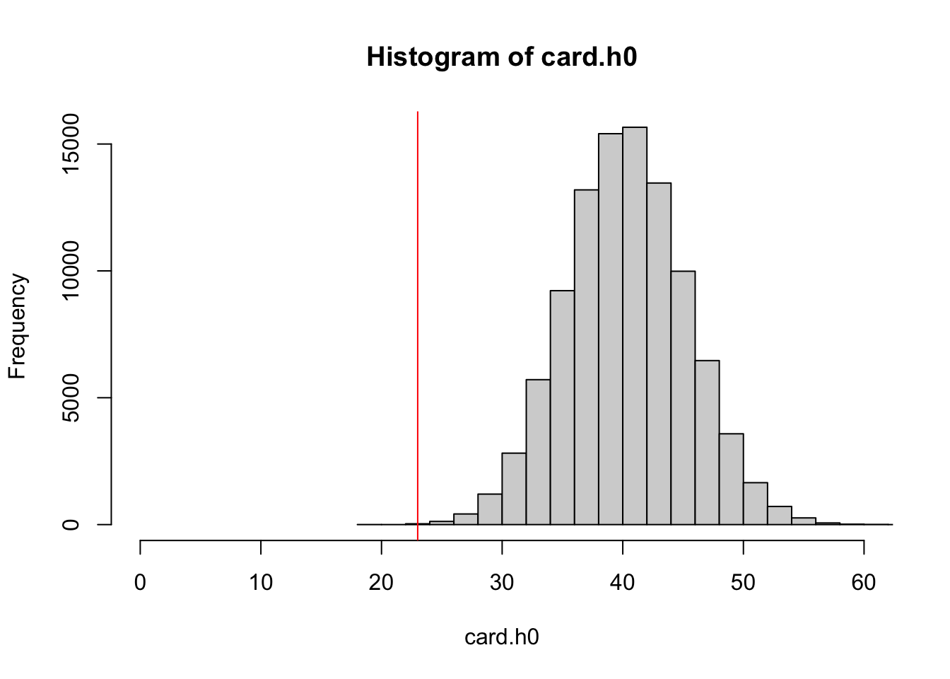
We can now calculate a p-value as the frequency of observed values under \(H_0\) which were more extreme than our observed values.
To make the calculation more robust, we add + 1 to both sides of the division.
(sum(emp.dupl >= card.h0) + 1)/(n.sim + 1)## [1] 0.0001299987Such an extreme value would be very unlikely, given that the \(H_0\) is true. We would therefore reject \(H_0\).
11.3 Under H1 (Power)
pacman::p_load(
  tidyverse, # for data wrangling and stuff...
  lme4,
  simr
  )
11.3.1 Background
Power is the probability of detecting an effect given that the effect is true. In practice, the concept of power is used to determine an appropriate sample size for an experiment under the assumption that the effect of interest (generally a [set of] model parameter[s]) is true and of a particular size.
In simple cases one can derive an analytic solution for such a probability. This is not always feasible as models grow more complex. In such cases it can be very handy to rely on monte-carlo simulations.
We would then like to know how probable it is under the alternative hypothesi (\(H_1\)) to detect a significant effect for the parameter of interest. Monte-carlo simulations produce random data according to the model we are interested in. Such a model has to be clearly specified. We then simulate data based on our \(H_1\), fit the model, and evaluate whether the parameter of interest was significant (i.e. detected). To approximate the probability of detecting an effect we calculate the frequency of finding a significant effect given a predefined number of simulations.
11.3.1.1 Example (two independent samples t-test)
Let’s use the model:
\(Y = \beta_0 + \beta_1*X + \epsilon\)
Where Y is the dependent variable, X represents control (x = 0) or experimental (x = 1) group, and \(\epsilon\) is the random error. \(\beta_0\) is then the mean of group 0, and \(\beta_1\) the difference in means.
This is the model formulation for a t-test.
Traditionally, we have the null hypothesis \(H_0: \beta_1 = 0\). To calculate power we need to assume a specific effect size under the alternative hypothesis, e.g: \(H_1: \beta = 0.4\). Of course, we also need to specify a significance level.
For the t-test the analytic solution is straightforward. Here, we explore a monte carlo simulation for the same problem and subsequently compare the results.
We start with simulating one data set of x and y, with a fixed n of 100 and \(\beta = 0.4\).
set.seed(237894) # to make results reproducible

n <- 100
beta.1 <- .4

# If experimental group is randomly assigned:
# x <- sample(0:1, n, replace = TRUE)
# if done like this, the group sizes are not neccessarily equal.
# For this example, we can use a fixed x, the order does not matter.
x <- rep(0:1, times = n/2)
x
## [1] 0 1 0 1 0 1 0 1 0 1 0 1 0 1 0 1 0 1 0 1 0 1 0 1 0 1 0 1 0 1 0 1 0 1 0 1 0
## [38] 1 0 1 0 1 0 1 0 1 0 1 0 1 0 1 0 1 0 1 0 1 0 1 0 1 0 1 0 1 0 1 0 1 0 1 0 1
## [75] 0 1 0 1 0 1 0 1 0 1 0 1 0 1 0 1 0 1 0 1 0 1 0 1 0 1# under H_1 we use the specified beta.1.
y <- beta.1*x + rnorm(n) # effect based on x + error
# under H_0 we would replace beta.1 with 0, and would be left with only the random error.
# y <- 0*x + rnorm(n)Now this looks as follows:
plot(y~as_factor(x))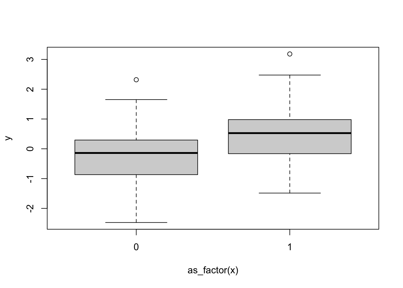
Here we can see that group 1 has a higher y value on average, but is it statistically significant?
summary(lm(y ~ x))##
## Call:
## lm(formula = y ~ x)
##
## Residuals:
## Min 1Q Median 3Q Max
## -2.27453 -0.65678 0.04281 0.49153 2.69333
##
## Coefficients:
## Estimate Std. Error t value Pr(>|t|)
## (Intercept) -0.1990 0.1445 -1.377 0.17156
## x 0.6884 0.2043 3.370 0.00108 **
## ---
## Signif. codes: 0 '***' 0.001 '**' 0.01 '*' 0.05 '.' 0.1 ' ' 1
##
## Residual standard error: 1.022 on 98 degrees of freedom
## Multiple R-squared: 0.1038, Adjusted R-squared: 0.09469
## F-statistic: 11.35 on 1 and 98 DF, p-value: 0.001078Yes it is.
We have now one instance of simulated data under \(H_1\). We would like to know how probable it is under \(H_1\) that a randomly simulated dataset yields a significant effect for the \(\beta_1\) coefficient. To approximate the probability we calculate the frequency of finding a significant \(\beta_1\) effect given a set number of simulations.
First, we write a function that always simulates a new set of data, fits a linear model and checks if the model was significant. For later use we let n be specified in the function call.
simulate_and_check <- function(n){
  x <- rep(0:1, n/2)
  y <- beta.1*x + rnorm(n) # effect based on x + error
  temp.dat <- data.frame(x, y)

  # fit model
  temp.lm <- lm(data = temp.dat, y ~ x)

  # check if effect was discovered in this one simulation
  # access p value and return TRUE if smaller than 0.05:
  summary(temp.lm)$coefficients["x",4] < .05
}
Lets see if the function works:
set.seed(237894) # same seed, same code, should yield TRUE
simulate_and_check(n = n)
## [1] TRUEWe can now repeat this simulation many times (n.sim times, to be precise).
We do this in a function, so we can do the same for different sample sizes.
n.sim <- 1000

# we want to get for each simulation the information whether we discovered the effect or not.
power <- function(n){
  # now we replicate this procedure n.sim times
  result <- replicate(n = n.sim, simulate_and_check(n))

  # we can now calculate power as the proportion of successful discoveries over total simulations (n.sim)
  sum(result)/n.sim
}power(n = n)## [1] 0.517Even better, we can now make the function take a whole vector of n’s and can find out how many people we need to get power = .8
power <- Vectorize(power) # this allows the power function to take a vector!

# specify n of interest:
n.vec <- seq(from = 10, to = 250, by = 20)

# get one result for each n
res.vec <- power(n.vec)

plot(x = n.vec, y = res.vec, type = "l")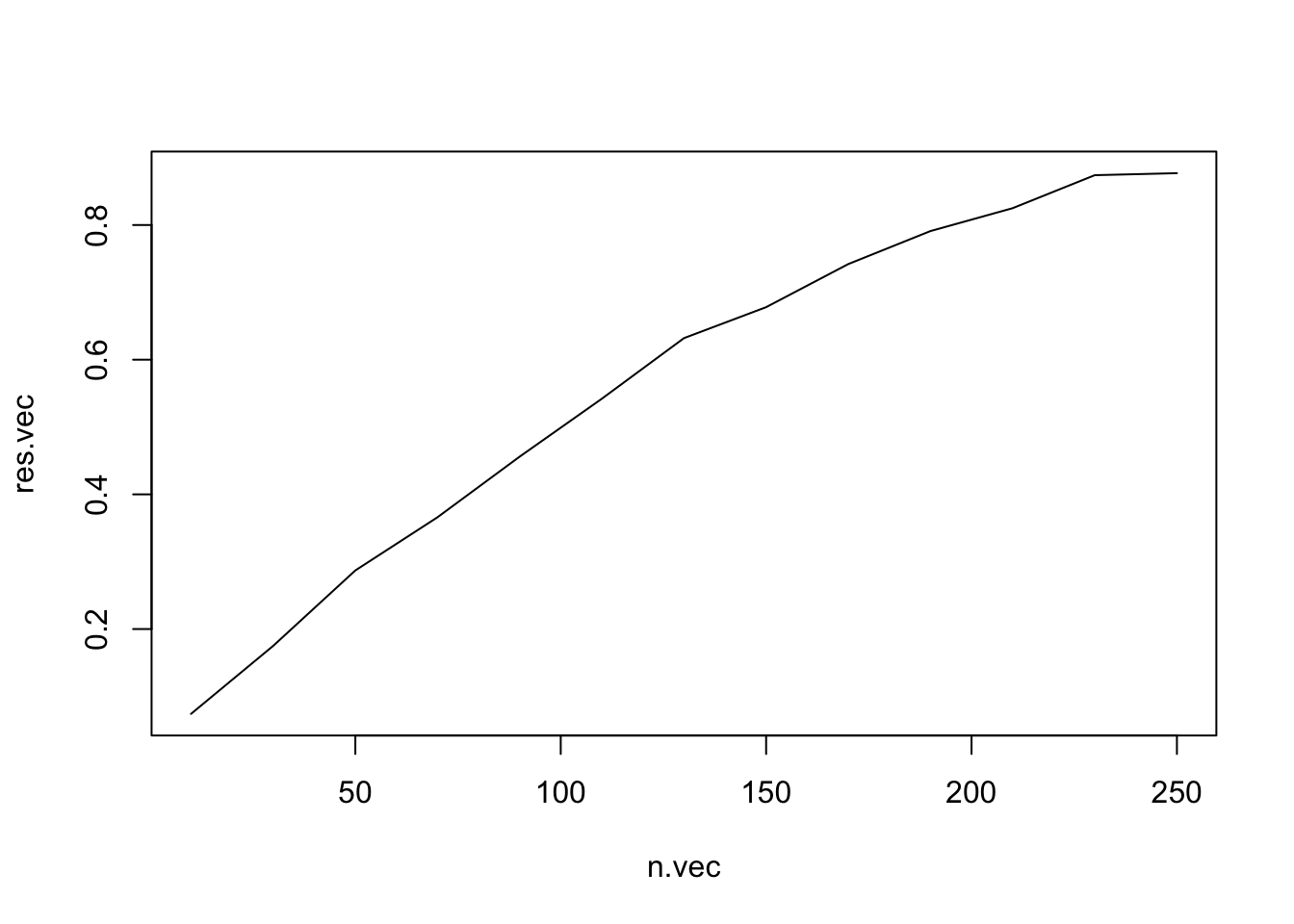
Analytic solution:
an.power <- power.t.test(n = n.vec/2, delta = beta.1, sd = 1, strict = TRUE)

# bind together
comp.dat <- data.frame(n = n.vec, simulated = res.vec, analytic = an.power$power)

# wide to long
comp.dat <- comp.dat %>%
  pivot_longer(names_to = "type",
               values_to = "power",
               cols = simulated:analytic)

head(comp.dat)
## # A tibble: 6 × 3
## n type power
## <dbl> <chr> <dbl>
## 1 10 simulated 0.074
## 2 10 analytic 0.0866
## 3 30 simulated 0.175
## 4 30 analytic 0.185
## 5 50 simulated 0.287
## 6 50 analytic 0.283# plot
ggplot(aes(x = n, y = power, color = type), data = comp.dat) +
geom_line()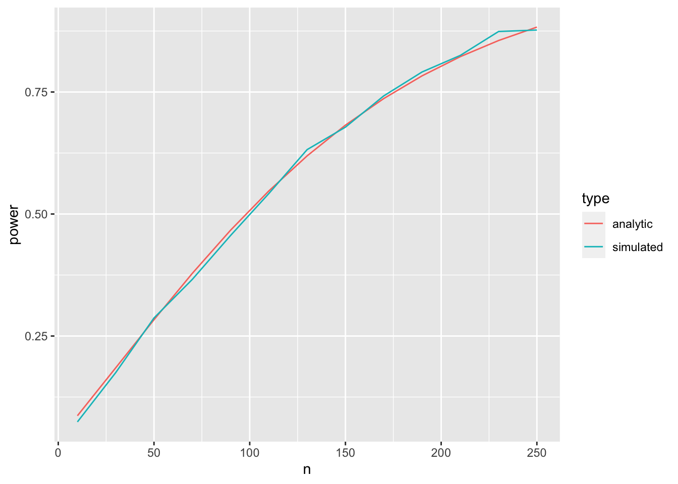
pretty close!
Some things to consider: Simulation takes much longer than the analytic solution. This can be a problem for complex models and large data sets. Also, the more times you simulate, the longer it takes. But with more simulations you get a higher accuracy for the power estimate.
We can see this by running the simulation with different number of simulations.
Here, we first do the simulation n.sim times, and then take various sub-samples of those simulations.
E.g. n.sim.5 has 0.5 times n.sim samples, so 500.
power.alternative <- function(n){
  # now we replicate this procedure n.sim times
  result <- replicate(n = n.sim, simulate_and_check(n))

  # we can now calculate power as the proportion of successful discoveries over total simulations (n.sim)
  c(n.sim = sum(result)/n.sim,
  n.sim.5 = sum(sample(result, size = n.sim*.5)) / (n.sim*.5),
  n.sim.2 = sum(sample(result, size = n.sim*.2)) / (n.sim*.2),
  n.sim.1 = sum(sample(result, size = n.sim*.1)) / (n.sim*.1),
  n.sim.05 = sum(sample(result, size = n.sim*.05)) / (n.sim*.05))
}
power.alternative <- Vectorize(power.alternative) # this allows the power function to take a vector!
# specify n of interest:
n.vec <- seq(from = 10, to = 250, by = 20)
# get one result for each n
res.vec.alternative <- power.alternative(n.vec)
res.vec.alternative <- rbind(n = n.vec, analytic = an.power$power, res.vec.alternative)
comp.dat.alternative <- as.data.frame(t(res.vec.alternative))
comp.dat.alternative <- comp.dat.alternative %>% gather(
key = "type", value = "sim.power", n.sim:n.sim.05
)ggplot(data = comp.dat.alternative, aes(x = n, y = sim.power, color = type)) +
geom_line() +
geom_line(aes(x = n, y = analytic), color = "black") +
theme_classic() +
geom_abline(slope = 0, intercept = .8, size = .3)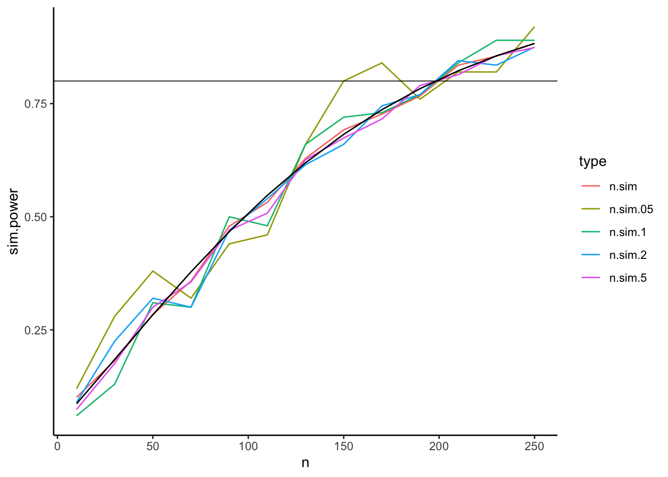
11.3.2 Power for mixed effects models
We compute power for mixed effects models using the simr package.
It allows for power simulations of lmer and glmer objects.
The package is relatively well documented.
Official information can be found here and here. (This)[https://humburg.github.io/Power-Analysis/simr_power_analysis.html] is a useful blogpost as well.
The data simulation are always based on a fitted lmer object.
Generally, we have to options to get a fitted lmer object.
Either we base it on available data, e.g. a pilot study or simulated data, or we can create the model from scratch using the makeLmer() function provided by the simr package.
Additionally, the simr package provides functionality to adjust sample sizes and parameters of a given fitted model.
11.3.2.1 Salary example
df <- read_csv(
  url("https://raw.githubusercontent.com/methodenlehre/data/master/salary-data2.csv")) %>%
  mutate(company = as.factor(company),
         sector = as.factor(sector),
         id = as_factor(1:nrow(.)))
## Rows: 600 Columns: 4## ── Column specification ────────────────────────────────────────────────────────
## Delimiter: ","
## chr (2): company, sector
## dbl (2): experience, salary##
## ℹ Use `spec()` to retrieve the full column specification for this data.
## ℹ Specify the column types or set `show_col_types = FALSE` to quiet this message.Fit the model
random.intercept.model <-  lmer(salary ~ experience + (1 | company),
                                   data = df, REML = TRUE)
We want to vary sample size in this model. To verify that the sample size has changed in exactly the way we want, we constucted a custom function to summarise the new data.
The easy version is to just look at the output of the getData() function from the simr package.
We do this here too, but then continue to summarise the data in a specific way.
custom.summary <- function(model){
  getmode <- function(v) {
   uniqv <- unique(v)
   uniqv[which.max(tabulate(match(v, uniqv)))]
  }

  getData(model) %>% group_by(company) %>%
  summarise(n = n(),
            mean.exp = mean(experience),
            mean.salary = mean(salary),
            sector = getmode(sector)
  ) %>% group_by(sector) %>%
  print() %>%
  summarise(n = n())
}
The custom.summary() function takes a fitted model as input, and outputs a summary of the getData() function output.
We can then, for example, directly look at a summary of the originally fitted data:
custom.summary(random.intercept.model)## # A tibble: 20 × 5
## # Groups: sector [2]
## company n mean.exp mean.salary sector
## <fct> <int> <dbl> <dbl> <fct>
## 1 Company 01 30 6.37 9588. Private
## 2 Company 02 30 6.13 9927. Private
## 3 Company 03 30 6.09 10808. Private
## 4 Company 04 30 4.71 7514. Public
## 5 Company 05 30 6.34 9764. Private
## 6 Company 06 30 5.1 7705. Private
## 7 Company 07 30 4.02 8727. Public
## 8 Company 08 30 5.71 8463. Private
## 9 Company 09 30 5.15 8036. Private
## 10 Company 10 30 5.21 9565. Public
## 11 Company 11 30 5.40 8193. Private
## 12 Company 12 30 4.91 9750. Public
## 13 Company 13 30 5.23 7938. Public
## 14 Company 14 30 4.70 7687. Public
## 15 Company 15 30 4.15 7487. Public
## 16 Company 16 30 4.88 8632. Public
## 17 Company 17 30 5.61 9450. Private
## 18 Company 18 30 5.03 8557. Public
## 19 Company 19 30 4.02 9116. Public
## 20 Company 20 30 5.04 7844. Private## # A tibble: 2 × 2
## sector n
## <fct> <int>
## 1 Private 10
## 2 Public 10We see that we get 20 companies with each 30 participants. 10 companies are in sector Public, 10 in sector Private.
We can then do a power simulation.
The function powerSim() chooses a parameter to calculate power for.
We can specify that ourselves, although in this case the function chooses correctly.
We set the parameter nsim (number of simulations) very low, as otherwise this takes too long.
powerSim(random.intercept.model, nsim = 20, test = fcompare(salary ~ 1))## Simulating: | |Simulating: |=== |Simulating: |====== |Simulating: |========= |Simulating: |============= |Simulating: |================ |Simulating: |=================== |Simulating: |======================= |Simulating: |========================== |Simulating: |============================= |Simulating: |================================= |Simulating: |==================================== |Simulating: |======================================= |Simulating: |========================================== |Simulating: |============================================== |Simulating: |================================================= |Simulating: |==================================================== |Simulating: |======================================================== |Simulating: |=========================================================== |Simulating: |============================================================== |Simulating: |==================================================================|## Warning in observedPowerWarning(sim): This appears to be an "observed power"
## calculation## Power for model comparison, (95% confidence interval):
## 100.0% (83.16, 100.0)
##
## Test: Likelihood ratio
## Comparison to salary ~ 1 + [re]
##
## Based on 20 simulations, (0 warnings, 0 errors)
## alpha = 0.05, nrow = 600
##
## Time elapsed: 0 h 0 m 1 s
##
## nb: result might be an observed power calculationNow, we have a huge sample size, so no wonder the power is very large.
We can use the extend() function to either extend or shrink data within a model along a variable.
Before, we had 20 companies. We can extend this to 60 companies:
random.intercept.model.2 <- extend(random.intercept.model,
                                   along = "company", n = 60)

custom.summary(random.intercept.model.2)
## # A tibble: 60 × 5
## # Groups: sector [2]
## company n mean.exp mean.salary sector
## <fct> <int> <dbl> <dbl> <fct>
## 1 a 30 6.37 9588. Private
## 2 b 30 6.13 9927. Private
## 3 c 30 6.09 10808. Private
## 4 d 30 4.71 7514. Public
## 5 e 30 6.34 9764. Private
## 6 f 30 5.1 7705. Private
## 7 g 30 4.02 8727. Public
## 8 h 30 5.71 8463. Private
## 9 i 30 5.15 8036. Private
## 10 j 30 5.21 9565. Public
## # … with 50 more rows## # A tibble: 2 × 2
## sector n
## <fct> <int>
## 1 Private 30
## 2 Public 30We now have 60 companies with each 30 employees.
On this extended model, we could again run the powerSim() function.
Similarly, we can extend the number of employees in total, if he have an id variable specified:
random.intercept.model.3 <- extend(random.intercept.model,
                                   along =  "id", n = 800)

custom.summary(random.intercept.model.3)
## # A tibble: 20 × 5
## # Groups: sector [2]
## company n mean.exp mean.salary sector
## <fct> <int> <dbl> <dbl> <fct>
## 1 Company 01 60 6.37 9588. Private
## 2 Company 02 60 6.13 9927. Private
## 3 Company 03 60 6.09 10808. Private
## 4 Company 04 60 4.71 7514. Public
## 5 Company 05 60 6.34 9764. Private
## 6 Company 06 60 5.1 7705. Private
## 7 Company 07 50 4.03 8814. Public
## 8 Company 08 30 5.71 8463. Private
## 9 Company 09 30 5.15 8036. Private
## 10 Company 10 30 5.21 9565. Public
## 11 Company 11 30 5.40 8193. Private
## 12 Company 12 30 4.91 9750. Public
## 13 Company 13 30 5.23 7938. Public
## 14 Company 14 30 4.70 7687. Public
## 15 Company 15 30 4.15 7487. Public
## 16 Company 16 30 4.88 8632. Public
## 17 Company 17 30 5.61 9450. Private
## 18 Company 18 30 5.03 8557. Public
## 19 Company 19 30 4.02 9116. Public
## 20 Company 20 30 5.04 7844. Private## # A tibble: 2 × 2
## sector n
## <fct> <int>
## 1 Private 10
## 2 Public 10We now have 800 employees and still 20 companies, but the employees are not uniformly distributed amongst the companies. It looks like the companies are topped up with employees in multiples of the original employee numbers.
We can also extend within id in company by 2, and then have each id twice in each company:
# each id is used twice.
random.intercept.model.4 <- extend(random.intercept.model,
                                   within =  "id + company", n = 2)

custom.summary(random.intercept.model.4)
## # A tibble: 20 × 5
## # Groups: sector [2]
## company n mean.exp mean.salary sector
## <fct> <int> <dbl> <dbl> <fct>
## 1 Company 01 60 6.37 9588. Private
## 2 Company 02 60 6.13 9927. Private
## 3 Company 03 60 6.09 10808. Private
## 4 Company 04 60 4.71 7514. Public
## 5 Company 05 60 6.34 9764. Private
## 6 Company 06 60 5.1 7705. Private
## 7 Company 07 60 4.02 8727. Public
## 8 Company 08 60 5.71 8463. Private
## 9 Company 09 60 5.15 8036. Private
## 10 Company 10 60 5.21 9565. Public
## 11 Company 11 60 5.40 8193. Private
## 12 Company 12 60 4.91 9750. Public
## 13 Company 13 60 5.23 7938. Public
## 14 Company 14 60 4.70 7687. Public
## 15 Company 15 60 4.15 7487. Public
## 16 Company 16 60 4.88 8632. Public
## 17 Company 17 60 5.61 9450. Private
## 18 Company 18 60 5.03 8557. Public
## 19 Company 19 60 4.02 9116. Public
## 20 Company 20 60 5.04 7844. Private## # A tibble: 2 × 2
## sector n
## <fct> <int>
## 1 Private 10
## 2 Public 10Or much more useful; just extend number of entries within companies:
# get more ids within company (I hope)
random.intercept.model.5 <- extend(random.intercept.model,
                                   within =  "company", n = 35)

custom.summary(random.intercept.model.5)
## # A tibble: 20 × 5
## # Groups: sector [2]
## company n mean.exp mean.salary sector
## <fct> <int> <dbl> <dbl> <fct>
## 1 Company 01 35 6.39 9595. Private
## 2 Company 02 35 6.24 10116. Private
## 3 Company 03 35 6.07 10827. Private
## 4 Company 04 35 4.71 7554. Public
## 5 Company 05 35 6.29 9649. Private
## 6 Company 06 35 5.16 7671. Private
## 7 Company 07 35 3.99 8619. Public
## 8 Company 08 35 5.76 8524. Private
## 9 Company 09 35 5.02 7969. Private
## 10 Company 10 35 5.23 9551. Public
## 11 Company 11 35 5.31 8045. Private
## 12 Company 12 35 4.88 9775. Public
## 13 Company 13 35 5.18 8020. Public
## 14 Company 14 35 4.55 7700. Public
## 15 Company 15 35 4.22 7514. Public
## 16 Company 16 35 4.81 8539. Public
## 17 Company 17 35 5.59 9444. Private
## 18 Company 18 35 5.04 8456. Public
## 19 Company 19 35 4.06 9046. Public
## 20 Company 20 35 5.08 7849. Private## # A tibble: 2 × 2
## sector n
## <fct> <int>
## 1 Private 10
## 2 Public 1011.3.2.1.1 Adjust effect sizes
When we have a fitted model we can adjust the effect sizes according to our needs.
We use the random.intercept.model.5 as an example.
fixef(random.intercept.model.5)["experience"] <- 150

summary(random.intercept.model.5)
## Linear mixed model fit by REML. t-tests use Satterthwaite's method [
## lmerModLmerTest]
## Formula: salary ~ experience + (1 | company)
## Data: df
##
## REML criterion at convergence: 10127.1
##
## Scaled residuals:
## Min 1Q Median 3Q Max
## -2.8109 -0.6884 0.0005 0.5980 3.8833
##
## Random effects:
## Groups Name Variance Std.Dev.
## company (Intercept) 614367 783.8
## Residual 1184502 1088.3
## Number of obs: 600, groups: company, 20
##
## Fixed effects:
## Estimate Std. Error df t value Pr(>|t|)
## (Intercept) 5964.18 229.41 48.00 25.997 < 2e-16 ***
## experience 150.00 27.21 589.48 5.514 5.26e-08 ***
## ---
## Signif. codes: 0 '***' 0.001 '**' 0.01 '*' 0.05 '.' 0.1 ' ' 1
##
## Correlation of Fixed Effects:
## (Intr)
## experience -0.615We can now check what the power would be for such a small effect size:
powerSim(random.intercept.model.5, nsim = 20)## Simulating: | |Simulating: |=== |Simulating: |====== |Simulating: |========= |Simulating: |============= |Simulating: |================ |Simulating: |=================== |Simulating: |======================= |Simulating: |========================== |Simulating: |============================= |Simulating: |================================= |Simulating: |==================================== |Simulating: |======================================= |Simulating: |========================================== |Simulating: |============================================== |Simulating: |================================================= |Simulating: |==================================================== |Simulating: |======================================================== |Simulating: |=========================================================== |Simulating: |============================================================== |Simulating: |==================================================================|## Power for predictor 'experience', (95% confidence interval):
## 100.0% (83.16, 100.0)
##
## Test: unknown test
## Effect size for experience is 1.5e+02
##
## Based on 20 simulations, (0 warnings, 0 errors)
## alpha = 0.05, nrow = 700
##
## Time elapsed: 0 h 0 m 5 sIt is still reasonably large.
But how many employees should we sample within the companies to get a power of 80%?
random.int.5.pc <- powerCurve(random.intercept.model.5, nsim = 60,
                               within = "company", progress = FALSE)
## boundary (singular) fit: see ?isSingular
## boundary (singular) fit: see ?isSingularThe powerCurve() function automatically selects 10 positions along the specified variable and simulates the power accordingly.
We can plot the object:
plot(random.int.5.pc)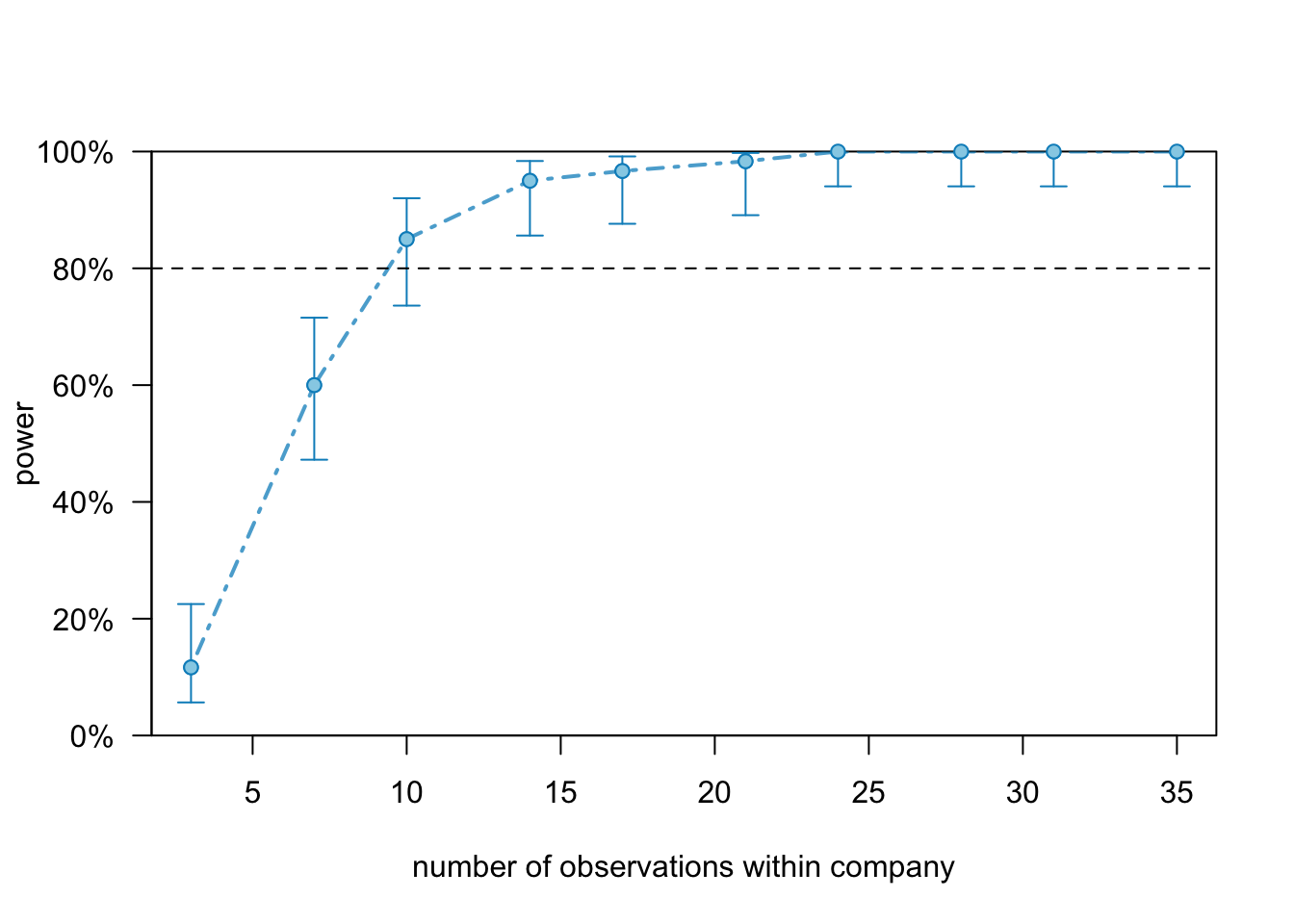
And see that we need 15 employees per company to get 80% power.
To get a better resolution around the number of observation within company we can specify break points in the powerCurve() function:
random.int.5.pc2 <- powerCurve(random.intercept.model.5, nsim = 60,
within = "company", breaks = 8:12, progress = FALSE)plot(random.int.5.pc2)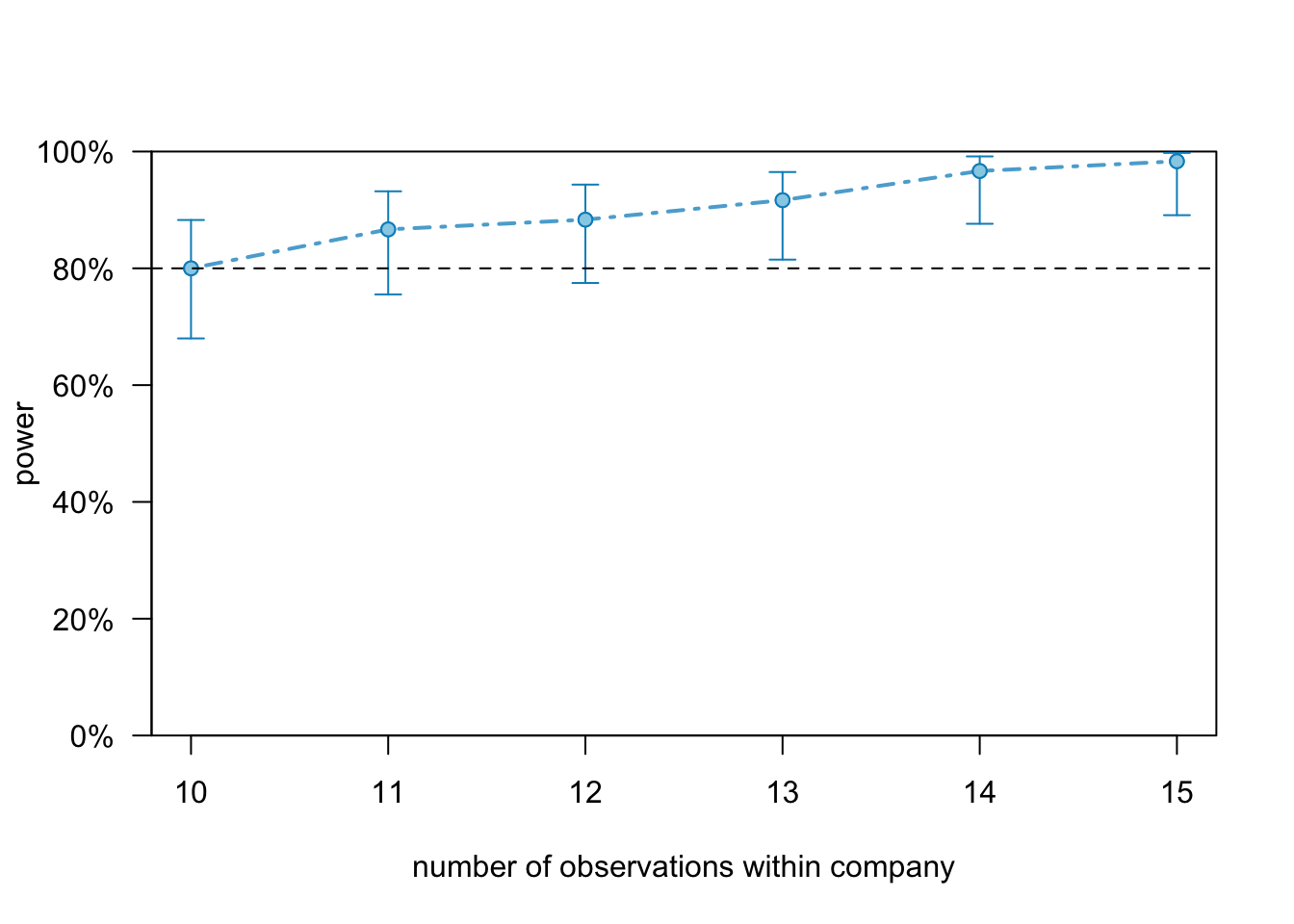
11.3.2.2 Repeated measures (from scratch)
We have a 2x2 within subjects design.
timepoint <- 1:2
condition <- 1:2
participant <- letters[1:10]
X <- expand.grid(timepoint = timepoint, participant = participant, condition = condition)
X
## timepoint participant condition
## 1 1 a 1
## 2 2 a 1
## 3 1 b 1
## 4 2 b 1
## 5 1 c 1
## 6 2 c 1
## 7 1 d 1
## 8 2 d 1
## 9 1 e 1
## 10 2 e 1
## 11 1 f 1
## 12 2 f 1
## 13 1 g 1
## 14 2 g 1
## 15 1 h 1
## 16 2 h 1
## 17 1 i 1
## 18 2 i 1
## 19 1 j 1
## 20 2 j 1
## 21 1 a 2
## 22 2 a 2
## 23 1 b 2
## 24 2 b 2
## 25 1 c 2
## 26 2 c 2
## 27 1 d 2
## 28 2 d 2
## 29 1 e 2
## 30 2 e 2
## 31 1 f 2
## 32 2 f 2
## 33 1 g 2
## 34 2 g 2
## 35 1 h 2
## 36 2 h 2
## 37 1 i 2
## 38 2 i 2
## 39 1 j 2
## 40 2 j 2Specify some fixed and random parameters.
b <- c(6, -.15, .002, .5) # fixed intercept and slope
V1 <- matrix(c(1, 0.5, 0.5, 1), 2) # random intercept and slope variance-covariance matrix
s <- 1 # residual standard deviation
scratch1 <- makeLmer(y ~ condition*timepoint + (timepoint|participant),
fixef=b, VarCorr=V1, sigma=s, data=X)
scratch1## Linear mixed model fit by REML ['lmerMod']
## Formula: y ~ condition * timepoint + (timepoint | participant)
## Data: X
## REML criterion at convergence: 117.1171
## Random effects:
## Groups Name Std.Dev. Corr
## participant (Intercept) 1
## timepoint 1 0.50
## Residual 1
## Number of obs: 40, groups: participant, 10
## Fixed Effects:
## (Intercept) condition timepoint
## 6.000 -0.150 0.002
## condition:timepoint
## 0.500Note that the y variable was not defined outside of the function makeLmer.
We an calculate power for the interaction effect by:
powerSim(scratch1, nsim = 20, test = fcompare(y ~ condition + timepoint), progress = FALSE)## Power for model comparison, (95% confidence interval):
## 10.00% ( 1.23, 31.70)
##
## Test: Likelihood ratio
## Comparison to y ~ condition + timepoint + [re]
##
## Based on 20 simulations, (0 warnings, 0 errors)
## alpha = 0.05, nrow = 40
##
## Time elapsed: 0 h 0 m 1 sWe estimate the power as 25%. Again, we can also expand the data to estimate power for more participants:
scratch2 <- extend(scratch1, along = "participant", n = 150)
# look at data to verify:
summary(getData(scratch2))
## timepoint participant condition y
## Min. :1.0 a : 4 Min. :1.0 Min. : 4.303
## 1st Qu.:1.0 b : 4 1st Qu.:1.0 1st Qu.: 5.940
## Median :1.5 c : 4 Median :1.5 Median : 6.629
## Mean :1.5 d : 4 Mean :1.5 Mean : 7.037
## 3rd Qu.:2.0 e : 4 3rd Qu.:2.0 3rd Qu.: 7.718
## Max. :2.0 f : 4 Max. :2.0 Max. :11.642
## (Other):576# redo power simulation
powerSim(scratch2, nsim = 50, fcompare(y ~ condition + timepoint), progress = FALSE)## Power for model comparison, (95% confidence interval):
## 80.00% (66.28, 89.97)
##
## Test: Likelihood ratio
## Comparison to y ~ condition + timepoint + [re]
##
## Based on 50 simulations, (50 warnings, 0 errors)
## alpha = 0.05, nrow = 600
##
## Time elapsed: 0 h 0 m 6 sWe get around 80 % power.
Again, we can investigate the powerCurve():
scratch.pc <- powerCurve(scratch2, test = fcompare(y~condition + timepoint),
                         nsim = 50, along = "participant", progress = FALSE)
plot(scratch.pc)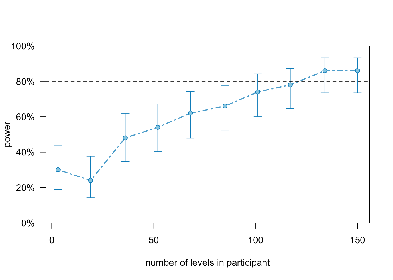
11.3.2.2.1 Adjusting random variance
We can modify the variance-covariance matrix similarly to the fixed effects. However, we must assign a matrix, not just a vector. The matrix we assign is the variance-covariance matrix. What the model prints out are the standard deviations and the correlation.
https://cran.r-project.org/web/packages/simr/vignettes/fromscratch.html \[\operatorname{cor}(x, y)=\frac{\operatorname{cov}(x, y)}{s d(x) \times s d(y)}\]
# define new VarCorr matrix
V2 <- matrix(c(0.5,0.05,0.05,0.1), 2)
V2
## [,1] [,2]
## [1,] 0.50 0.05
## [2,] 0.05 0.10# assign it
VarCorr(scratch2) <- V2We should now get in the model print out:
# random intercept sd:
(int.sd <- sqrt(0.5) %>% round(3))
## [1] 0.707# random slope sd:
(slope.sd <- sqrt(0.1) %>% round(3))## [1] 0.316# correlation
(0.05/(int.sd*slope.sd)) %>% round(3)## [1] 0.224# lets see:
scratch2## Linear mixed model fit by REML ['lmerMod']
## Formula: y ~ condition * timepoint + (timepoint | participant)
## Data: X
## REML criterion at convergence: 117.1171
## Random effects:
## Groups Name Std.Dev. Corr
## participant (Intercept) 0.7071
## timepoint 0.3162 0.22
## Residual 1.0000
## Number of obs: 40, groups: participant, 10
## Fixed Effects:
## (Intercept) condition timepoint
## 6.000 -0.150 0.002
## condition:timepoint
## 0.500Looks correct.
We can also modify the residual variance using the scale() function.
scale(scratch2) <- 1.3

scratch2
## Linear mixed model fit by REML ['lmerMod']
## Formula: y ~ condition * timepoint + (timepoint | participant)
## Data: X
## REML criterion at convergence: 117.1171
## Random effects:
## Groups Name Std.Dev. Corr
## participant (Intercept) 0.9192
## timepoint 0.4111 0.22
## Residual 1.3000
## Number of obs: 40, groups: participant, 10
## Fixed Effects:
## (Intercept) condition timepoint
## 6.000 -0.150 0.002
## condition:timepoint
## 0.500